Dynamic Image Analysis: Principles, Data Quality, and Applications
Introduction
Dynamic image analysis (DIA) is a sophisticated analytical technique used to characterize and measure the size, shape, and other morphological properties of particles or objects within a sample. It enables simultaneous analysis of multiple size- and shape-dependent features of every particle within the detected population of particles, one by one. DIA has proved itself as a viable R&D and quality control method across various industries, including pharmaceuticals, food, chemicals, materials science, environmental sciences, and biotechnology. In this article, we will explore the principles, methodology, applications, and advantages of dynamic image analysis in detail.
Principles of Dynamic Image Analysis
To understand how DIA works it's essential to grasp the underlying principles, process steps, and components of the technique.
Sample preparation
The process begins with the preparation of a representative sample. This sample can consist of various materials, such as powders, granules, suspensions, or even biological specimens like cells. The sample is dispersed in a suitable medium, which can be a liquid or a gas, depending on the application. Ensuring proper sample preparation and proper sampling is crucial to obtaining accurate and representative data.
DIA measurement results are intrinsically number-based but can be recalculated into surface- or volume-based results. Hence, it is of the utmost importance to prepare – and measure – a high enough number of particles. The minimum sample amount is defined by the requested standard deviation of the result and the size distribution itself. The expected standard deviation of the calculated size distribution depends on the number of measured particles. Typically, more than 1,000,000 (one million) particles are needed to achieve a maximum error below 1%.
Instrumentation and image capture
Dynamic image analysis relies on specialized instruments called dynamic image analyzers or particle analyzers. These instruments are designed to capture high-speed images of particles in motion. Key components of a typical dynamic image analyzer include:
- High-speed camera: A high-speed camera with a fast frame rate is used to record a sequence of images. These cameras can typically capture hundreds of images per second, enabling the observation of rapid particle movements.
- Lighting system: Adequate illumination is critical for capturing clear images of particles. The lighting system provides uniform and consistent illumination to ensure accurate analysis.
- Sample chamber: The sample is placed in a chamber where it is continuously agitated or dispersed. Various mechanisms, such as vibration, airflow, or fluid circulation, can be employed to keep the particles in motion.
- Optics: The optical system includes lenses and filters that focus and filter the light before it reaches the camera sensor.
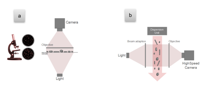
As a technique, DIA shares certain similarities with both traditional light optical microscopy (LOM) and static image analysis (SIA). DIA also uses light and optics but differs from LOM and SIA as a) particles are in motion and constantly exchanged during the measurement, b) particles are randomly oriented towards the camera, and c) particles are detected and analyzed automatically. For these reasons, DIA can include very large numbers of particles in each single measurement, which is necessary to achieve good statistical quality of the resulting distributions (Figure 1).
DIA typically covers a very wide measuring range. The lower end of the measurement range is defined both by the camera sensor pixel size and the magnification provided by the objectives. Litesizer DIA has a resolution (minimum pixel size) of 0.5 µm, which also constitutes the lower limit of its measurement range. The upper detection limit is defined by:
- The mechanical design of both the measurement cell and dispersion unit.
- The pixel size: The smaller the pixel size, the smaller the camera frame.
- The physical size of the camera frame: According to ISO 13322-2[1], the maximum size is equal to one-third of the lesser dimension of the field of view.
Due to optical limitations, even when a high-resolution camera is in use, it is possible to cover only a limited measurement range using a single optical objective – typically three orders of magnitude. Expanding it to four or five orders requires performing the measurement using two or more objectives and merging the datasets.
Image processing
Once dispersed, the particles travel through the measurement zone using gravity, air pressure, or in a moving carrier liquid. Backlight illumination (shadow projection) is used to produce greyscale images of the particles. These projections are converted into binary images to determine the particles' contours, which can then be used for shape and size analysis.
The heart of DIA lies in the analysis of the captured images. Advanced image analysis algorithms and software are used to process the images and extract relevant information about the particles. The analysis includes several key steps:
- Particle detection: The software identifies and locates individual particles or objects within each captured frame.
- Binary image system
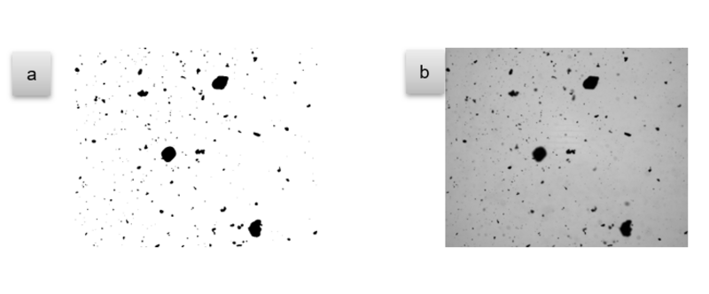
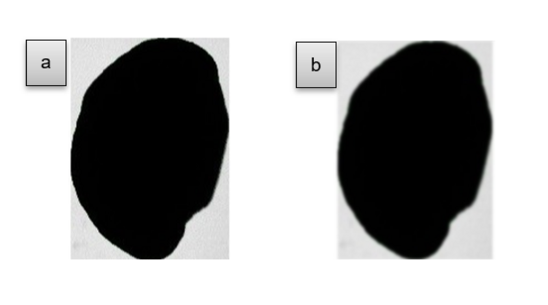
Simple systems may use a thresholding method to generate binary images of the frame. With this method, each pixel is replaced by a black pixel if the grey value is larger than a fixed value called threshold, or by a white pixel for grey values smaller than the threshold (and the other way around to define the background). This procedure generates black particle projections on a white background (Figure 2a). To account for illumination inhomogeneities, dynamic threshold values are usually applied. The change of the threshold value depends on the background and the local contrast conditions at the position of the considered particle. - Grayscale image system
More advanced systems use a grayscale as a source of information. Combined with the analysis of the neighboring pixels, this results in greater sensitivity to the fine features on the surface of particles or objects (Figure 2b).
- Binary image system
- Tracking: The software tracks the movement of each particle across successive frames, allowing the determination of particle trajectories.
- Attribute measurement: Various particle attributes are measured, including size, shape, velocity, and other morphological characteristics.
- Data processing: The data obtained from the image analysis are processed to generate size and shape distributions and other relevant metrics.
Instrument calibration and validation
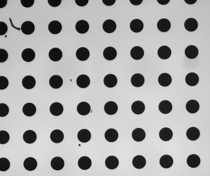
DIA instruments have to be calibrated to convert pixels into SI length units (e.g., µm). For the calibration, a certified, static target with structures of known size is used. In the case of Litesizer DIA, the distance between the center of the dots is determined, and the mean distance is used to calculate the corresponding value, typically expressed in micrometers (Figure 3).
For the validation of the measurement system, moving particles of a certified reference material with a known diameter have to be used.
Lower and upper size limits
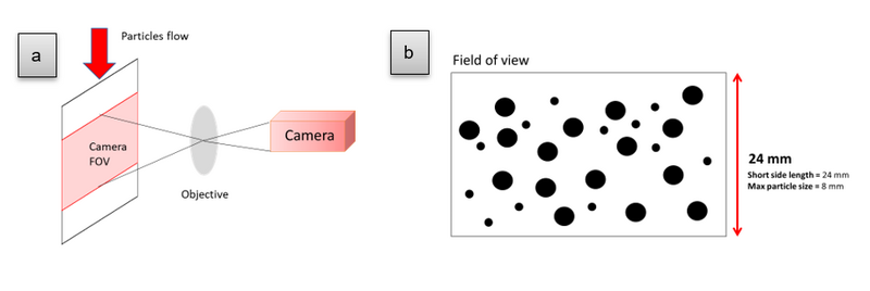
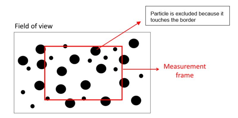
According to ISO 13322-2, at least three pixels are required, aligned in one dimension, for acceptable sizing. At least nine pixels are required in one dimension for reliable shape analysis. The maximum particle size should be limited to one-third of the shortest side of the field of view. Exceeding this limit will significantly increase the risk of the particle’s image touching one of the measurement frame’s edges (Figure 4). It means that particles smaller than one-third the size of the shorter side of the field of view can be correctly measured.
Particle images cut by the edges of the measurement frame
If all particle images that appear in the frame are accepted for measurement, the accuracy of the measurement will be impaired because some particle images will inevitably be cut by the frame’s edges. To overcome this, particle images that are touching the edges must be excluded from the analysis (Figure 5). However, the probability that a particle’s image touches the edges increases with its size, also potentially skewing the distribution. To counter this effect, a statistical correction must be applied by the algorithm generating the particle size distribution.
Sources of Uncertainty
Potential sources of uncertainty during DIA-based measurement include [2]:
- Optical distortion errors
- Depth of field of camera focus
- Motion blur (particle velocity and integration time)
- Contaminations (e.g., by air bubbles in the carrier liquid)
- Overlapping of particle images
- Particle orientation
- Background correction (for non-uniformity of illumination)
Overlapping particle images
It is a prime requirement of the method that measurements must be performed on isolated particles. The frame coverage value must be low enough to limit the number of particles that are seemingly overlapping on the image because they are moving simultaneously in different planes within the depth of field. The frame coverage is a simple parameter helping to adjust particle feed and is defined as a percentage of the image area that is obscured by the projection of all particles. For Litesizer DIA, the recommended frame coverage should not exceed 0.5%, although acceptable values can vary greatly depending on particle size.
Blurred particle images
The particles are imaged with maximum sharpness of their edges if they are positioned in the so-called object plane. However, the images can be accepted for analysis if the edges have a minimum sharpness. This threshold sharpness defines a depth of field where particles are imaged sharply enough (Figure 6). Furthermore, this depth of field defines a measurement volume that includes all measured particles. Particles outside of the depth of field are too blurred for analysis and have to be excluded from the measurement.
Motion blur
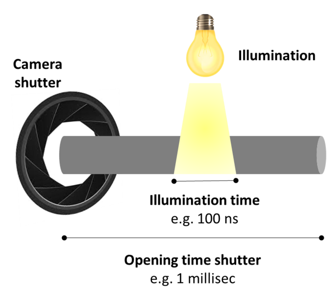
The exposure time of the imaging system is usually defined by the light pulse length (strobe light). The pulse length has to be short enough to avoid significant motion blur, even for the fastest particles (Figure 7).
For Litesizer DIA, the opening time of the shutter is one millisecond, and the exposure time (illumination time) is around 100 ns (Figure 8).
Parameters Measured by Dynamic Image Analysis
DIA enables the measurement of a wide range of parameters related to particles or objects within the sample. These parameters provide detailed insights into the sample's characteristics and behavior. Bulk properties, such as density, flowability, ballistics, and many others, are related not only to particle size but also to particle shape.
Multiple size and shape parameters can be measured by DIA, and the most commonly used ones are presented in Table 1 and Table 2.
A single universal parameter applicable to every application does not exist, so the parameters most relevant to a specific sample must be selected carefully. Systems offering multiple, different size and shape parameters and maximum flexibility and customization are therefore a must.
Each particle can be categorized by multiple parameters at the same time, creating a multi-dimensional room. Nevertheless, the most practical approach for a user is taking two parameters, e.g., sphericity vs. particle size, to obtain a matrix. This allows us to quickly get an overview of the particles contained in the sample. The four corners show small spherical, small elongated, large spherical, and large elongated particles. Between the outermost edges and corners, the parameters vary gradually, showing also particles that do not represent extreme cases.
In theory, a third filtering parameter could be added, e.g., irregularity, resulting in a 3D cube, cuboid, or other 3D structure. One edge could represent small elongated irregular particles, another one large elongated regular particles, and then small spherical irregular particles, etc. Adding a fourth parameter, e.g., convexity, would result in a 4D structure, which is already difficult to represent .
Particle size
One of the fundamental measurements in DIA is particle size. The technique can accurately determine the dimensions of individual particles or objects within the sample. Typically, particle size is represented as either a mean size value or a size distribution, which shows the relative abundance of particles at different size ranges. Table 1 details how some of the most commonly used size parameters are calculated.
Table 1: Examples of size parameters measured with DIA. CC BY 4.0 licensed
| Size parameters | ||
| Parameter | Description | Schematic representation |
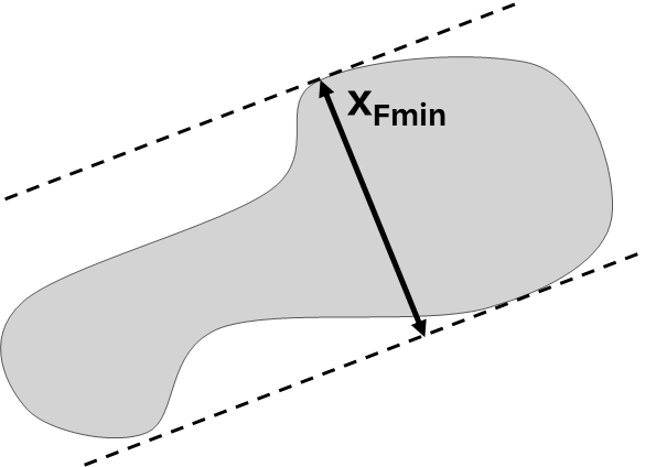
| xFmin Minimum Feret diameter |
The shortest distance between two parallel planes tangent to the contour of the particle. xFmin in particle analysis reflects the diameter of particles passing through sieves, especially irregular or bulky ones, and is useful for determining minimum diameters. However, it often underestimates particle size, skewing distributions lower due to sensitivity to minor surface features like protruding fibers. Notably, xFmin is not always perpendicular to xFmax. |
  |
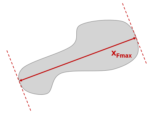
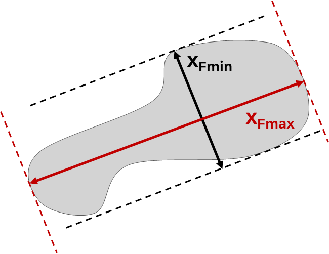
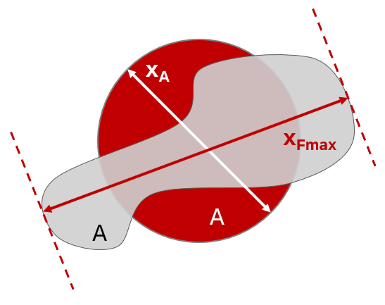
| xFmax Maximum Feret diameter |
The largest distance between two parallel planes tangent to the contour of the particle. The xFmax often skews the particle size distribution (PSD) towards higher values, potentially overestimating particle sizes. Small surface features, like minor protrusions, can significantly impact measurements. Misalignment with xFmin can further distort size estimations, highlighting the need to account for these effects for accurate particle size analysis. |
 |
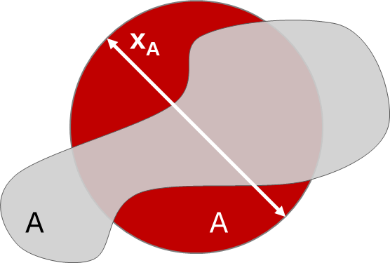
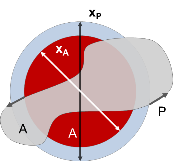
| xA Projected area equivalent diameter |
Diameter of a sphere with the same projected area (A) as the particle’s projection. xA=√(4A/π ) The xA is used for calculating volume- or surface-based size distributions and comparing cross-sectional sizes of particles with varying shapes. It is particularly useful for tracking changes from processes like wear or abrasion. Unlike Feret diameters, it cannot be directly compared to sieve analysis as it ignores particle outlines or shapes but remains effective for sizing agglomerates. |
 |
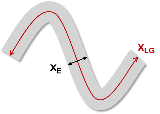
| xLG and xE Geodesic length and thickness |
Approximations for geodesic length and xE of very long and concave particles, such as fibers. The following equations are used for an area- and perimeter-equivalent rectangle: A= xLG × xE P=2(xLG+xE) The thickness (xE) measures a particle's average width, calculated as the average distance between parallel tangents across multiple orientations. xLG and xE are crucial for analyzing elongated or irregular particles like fibers and flakes. xLG determines the effective length of curved fibers, aiding in predicting their passage through sieves. xE measures flake thickness using image filtering techniques. Together, these parameters enhance the precision of particle size analysis for non-geometric shapes, ensuring accurate length and thickness measurements. |
 |
|
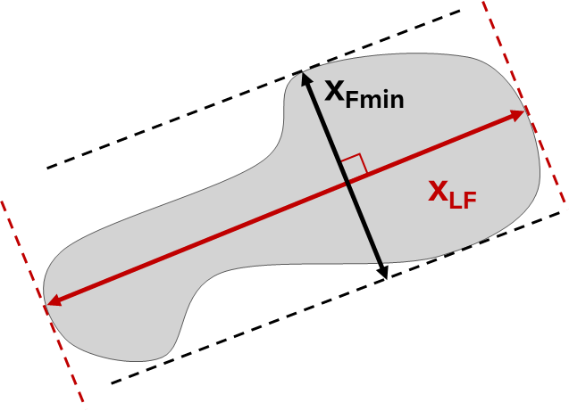
xLF Length |
The length (xLF) refers to the Feret diameter perpendicular to the minimum Feret diameter. It is a straightforward measure of the maximum dimension of irregularly shaped particles.
The length parameter (xLF) is essential for measuring particle dimensions, especially for elongated or irregular shapes. Unlike xFmax, which measures the maximum Feret diameter in any orientation, xLF is always perpendicular to xFmin and reflects the particle's longest dimension. It is always less than or equal to xFmax and is particularly useful for filtering and characterizing elongated objects. In quality control, xLF helps ensure uniform pellet lengths and maintains consistent particle dimensions in industrial and research settings. The xA exhibits insensitivity to the shape of the particle itself, focusing instead on the projected area, which can limit its applicability in scenarios where shape details are critical for analysis. |
 |
| Axes of the Legendre Ellipse (xLmin, xLmax) | The axes of the Legendre Ellipse approximate an irregular particle's shape with a best-fit ellipse, simplifying complex shapes in image analysis. This method preserves key details about a particle’s size, shape, and orientation while integrating convex areas and the center of mass. However, it tends to overlook minor surface irregularities. | 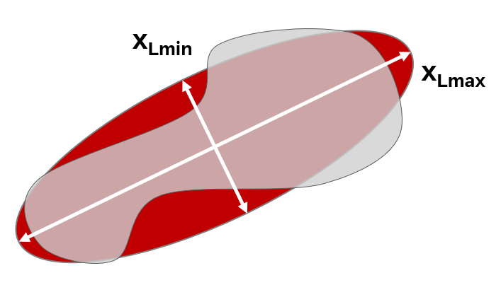 |
Particle shape
DIA provides information about the shape of particles or objects. Parameters like aspect ratio, circularity, elongation, and roundness can be used to quantify the shape characteristics of individual particles. Examples may be found in Table 2: Examples of shape parameters measured with DIA.
Table 2: Examples of shape parameters measured with DIA. CC BY 4.0 licensed
| Shape parameters | ||
| Aspect ratio |
The ratio of the minimum and maximum Feret diameters. It ranges from 0 to 1 (sphere). |
 |
| Elongation or eccentricity | The elongation of the particle is calculated as the ratio between thickness and geodesic length. It ranges from 0 to 1 (sphere). Elongation=xE/xLG Elongation measures how stretched a particle is, defined as the ratio of the difference between the major and minor axes to the major axis. The smaller the elongation values, the higher the elongation. It highlights a particle’s deviation from circularity and is useful for characterizing shapes. Insensitive to waviness or curvature, it effectively identifies fibers or flakes with specific length-to-width ratios. |
 |
| Circularity and form factor | The degree to which the particle (or its projection area) is similar to a circle, considering the smoothness of the perimeter (P). It ranges from 0 to 1 (sphere). Circularity = √(4πA/P2)=xA/xP Form factor=Circularity2=4πA/P2=(xA/xP)2 A circularity value of 1 indicates that the particle is perfectly circular. Values less than 1 suggest that the particle is not perfectly circular, with lower values indicating more irregular or elongated shapes. The form factor, also known as the shape factor, expresses the same relationship without the square root and quantifies how efficiently the particle's perimeter encloses its area. A value of 1 corresponds to a perfect circle, while lower values indicate increasingly irregular shapes. The form factor is particularly useful when the population of interest exhibits a high degree of sphericity, allowing small differences between very spherical particles to be resolved. |
 |
| Extent or bulkiness |
The ratio of particle area to the product of xFmax and xFmin defines extent, with a maximum value of 1 for fully stretched fibers, decreasing as they coil. Extent=A/(xFmax × xFmin) Elongation distinguishes rectangular shapes from irregular or spherical ones. A value of 1 identifies stretched fibers, rectangles (xFmin and xFmax perpendicular), or rhombuses (non-perpendicular), relying on xFmin and xFmax and being sensitive to protrusions. |
 |
| Ellipse ratio / elliptical shape factor |
The ellipse ratio incorporates the relationship between the lengths of the axes of the Legendre Ellipse. Ellipse ratio=xLmin/xLmax This parameter ranges from 0 to 1, with 1 representing a perfect sphere. It is highly sensitive to the distribution of area within the particle, effectively integrating the influence of convex areas and the position of the mass center. However, it tends to overlook surface irregularities. |
 |
| Solidity |
The measure of the overall concavity of a particle is calculated as the ratio between the area of the particle (A) and the area of the convex hull (AC). It ranges from 0 to 1 (sphere).
Solidity=A/AC This parameter is valuable for distinguishing between curved or undulating objects, such as fibers, and straight or bulky objects. It exhibits low sensitivity to variations in perimeter measurements. However, even minor protrusions from the overall bulk shape can significantly reduce its value. |
 |
| Irregularity |
It describes the relationship between the diameter of the maximum inscribed circle (di,max) and that of the minimum circumscribed circle (dc,min). It ranges from 0 to 1 (sphere).
Irregularity=di,max/dc,min This parameter is highly sensitive to surface irregularities, making it effective for identifying such features. Moderately sensitive to area distribution, it offers an alternative to circularity and form factor metrics. For fibers or elongated objects, it yields low values, reflecting their shape, and is valuable for characterizing and filtering particles by surface morphology in scientific and industrial contexts. |
 |
| Compactness |
The degree to which the particle (or its projection area) is similar to a circle, considering the overall form of the particle. It ranges from 0 to 1 (sphere).
Compactness=√(4A/π)/xFmax=xA/xFmax Compactness, highly sensitive to minor protrusions due to its reliance on xFmax, is useful for comparing particles with similar areas but differing imperfections. It effectively identifies particles with secondary shapes, like satellites on round particles, critical for characterizing surface morphology and attachments in additive manufacturing. |
 |
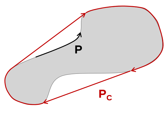
| Convexity |
The ratio between the perimeter of the convex hull (envelope) bounding the particle and the perimeter of the particle itself. It ranges from 0 to 1 (sphere).
Convexity=PC/P This parameter distinguishes bent or wavy objects like fibers from straight ones by analyzing shape characteristics. With limited sensitivity to surface area changes, it focuses on convex regions, making it a robust tool for shape analysis in scientific and industrial applications. |
 |
Particle velocity
By tracking the movement of particles in the frame sequence, DIA can calculate the velocity of particles. This information is valuable for understanding particle dynamics and behavior within the sample. Furthermore, this information is often used to create so-called “velocity correction curves.” These curves are designed to correct the measurement error originating from particles that, although they are being accelerated by the same means, are moving at different speeds. If not corrected, this error may lead to over- or under-representation of certain subpopulations of particles in the measured sample.
Image parameters
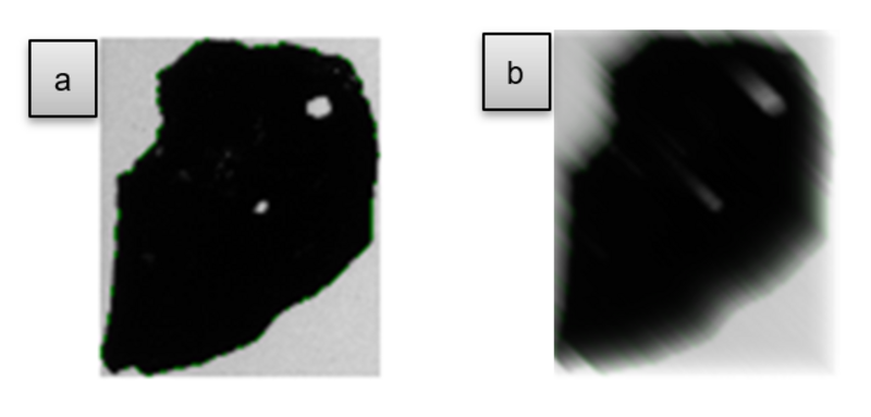
Image sharpness
The sharpness of a particle's contour in an image is determined by the gradient of the greyscale value in the direction perpendicular to the contour, averaged over the entire contour. For a particle that is sharply imaged (b), the greyscale value changes rapidly from high (bright) to low (dark) as one moves from the background toward the particle's center. Consequently, the gradient of the greyscale value and the sharpness parameter are both high. In contrast, for a blurred image (a), the gradient of the greyscale value and the sharpness are lower. Sharpness is not an inherent property of the particle itself, but rather it depends on the imaging optics. Specifically, it is influenced by the relative position of the particle to the depth of field of the imaging optics. This parameter is useful for filtering out blurred particle images.
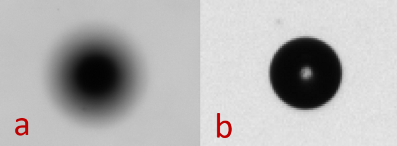
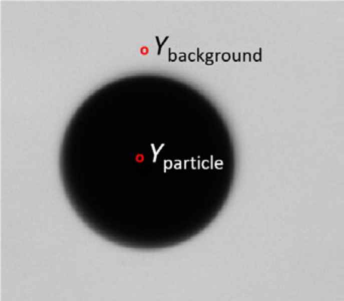
Image contrast
This parameter indicates the contrast of a particle image by measuring the difference in greyscale value (Y) between the background near the particle (Ybackground) and the area within the particle (Yparticle). The contrast value ranges from 0 to 1, where 1 represents a completely black particle.
$\text{Contrast} = \frac{Y_{\text{background}} - Y_{\text{particle}}}{Y_{\text{background}}}$
This parameter is particularly useful when analyzing fine features on particle surfaces is important. Additionally, it is valuable for selecting photos for reporting or scientific publication.
Applications of Dynamic Image Analysis
DIA has a wide range of applications, across various industries and scientific disciplines. Some notable applications include:
- Food industry
- Measuring the size and shape of food particles and ingredients, such as flour, sugar, and powdered milk.
- Analyzing the dispersion of additives and flavorings in food products.
- Analyzing coffee grounds and beans.
- Pharmaceuticals
- Analyzing the size and shape of drug particles in formulations.
- Monitoring the quality and uniformity of tablet coatings.
- Studying the behavior of active pharmaceutical ingredients (APIs) in suspensions.
- Environmental sciences
- Analyzing natural particles like sand, soil, and sediment in aquatic ecosystems.
- Studying the movement and transport of particles in air and water.
- Biotechnology
- Analyzing cell cultures to measure cell size and morphology.
- Monitoring the behavior of particles in bioprocesses, such as fermentation and cell culture.
- Manufacturing
- Studying the roundness of particles in battery materials.
- Analyzing the size and shape of cement (detailed below).
- Abrasives (detailed below).
- Additive manufacturing (detailed below).
Cement
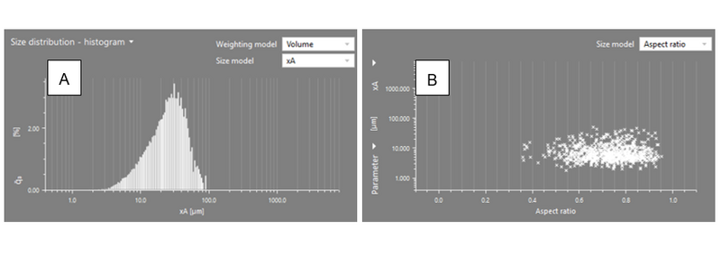
The quality of cement is strongly dependent upon the size and shape of its particles, which affect its surface area, compression strength, and curing time. Particles that are too fine cause an exothermal setting in the final product, while particles that are too large do not fully hydrate. Cement flowability and water demand may vary drastically between regular (spherical) and irregular particles. In fact, more regular particles hydrate faster.
An exemplary result for a cement sample is shown in Figure 9. The size distribution based on the xA size model is monomodal and broad, with the major part of the population ranging from 5 μm to 60 μm (Figure 9A). The aspect ratio displayed in Figure 9B shows that most of the particles have an aspect ratio close to 1, indicating a spherical shape.
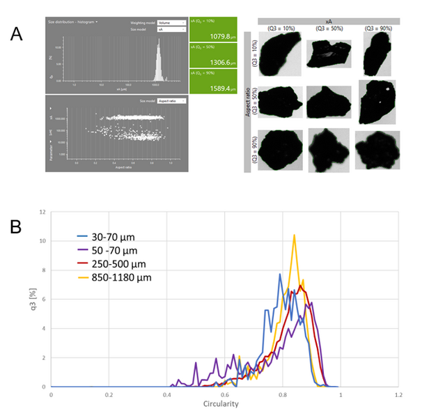
Abrasives
Abrasives include different types of materials, such as metals, ceramics, and polymers. They are used to polish and smooth the surface of metallic, plastic, or ceramic components. Their hardness, size, and shape all have an impact on the ultimate abrasive performance. Besides the aspect ratio, the shape parameter ‘circularity’ is of particular interest for abrasives. As displayed in Figure 10A, the size parameters as well as the aspect ratio/xA overview are by default shown after the measurement. In the analysis window, the circularity distribution can also be listed and evaluated. Interestingly, the circularity distribution (Figure 10B) shows that, even though the four abrasive samples tested have very different particle sizes, they all have a very similar shape distribution.
Additive manufacturing
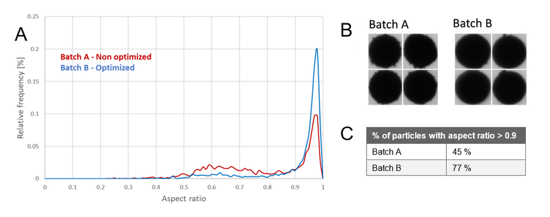
Most metal-based additive manufacturing (or 3D printing) technologies rely on metallic powders as a feedstock material. Since the quality of the powder used directly influences the quality of printed parts and printing speed, it is crucial to monitor its properties. The influence of the powder quality can be the most prominent in powder bed techniques, where the powder should have a high packing density and form smooth layers, usually in the range of 25 µm to 100 µm. Ultrasonic atomization is a liquid-to-solid process for the production of metallic powder, which uses ultrasonic vibrations to create the powders. The controlled atmosphere inside the atomization chamber will have an impact not only on the particle size but also on the shape. Metallic additive manufacturing expects a feedstock consisting of perfectly spherical particles. Elongated particles are difficult to separate after production and can therefore introduce irregularities into the powder bed. Figure 11 shows how the optimized conditions of the atomization process used for sample B increase the sphericity (aspect ratio close to 1) and reduce the characteristic flaky oxidation layer around the particle.
Advantages of Dynamic Image Analysis
Dynamic image analysis offers several advantages that make it a valuable tool in particle characterization:
- High sensitivity
- DIA is highly sensitive and can detect even minor changes in particle properties. This sensitivity is crucial for quality control and research applications where precision is paramount.
- DIA has a resolution of a single particle. This means that even a single outlier particle within a large population can be detected, provided that enough particles are analyzed.
- Shape analysis
- It is the only method providing an abundance of shape descriptors in addition to size parameters.
- Direct measurement
- DIA is based on direct observation, making it easy to verify the results by simply checking the images.
- Comprehensive data
- DIA provides a wealth of information about particles, including size, shape, velocity, and more. This comprehensive data allows for a deeper understanding of particle systems.
- Wide applicability
- DIA can be applied to a broad range of materials and sample types, making it a versatile technique that is suitable for diverse industries and research fields.
- Non-destructive
- DIA is a non-destructive technique, meaning it does not alter or damage the particles being analyzed. This is important in applications where sample integrity must be preserved.
Bibliography
[1] International Standard Organization, ISO 13322-2:2021. Particle size analysis. Image analysis methods, Part 2: Dynamic image analysis methods, 2021.
[2] J. G. Whiting, V. N. Tondare, J. H. J. Scott, T. Q. Phan, and M. A. Donmez, "Uncertainty of particle size measurements using dynamic image analysis," CIRP Annals, vol. 68, pp. 531-534, 2019.
Further Reading
- Application report on Dynamic Image Analysis of Cement
- Application report on Dynamic Image Analysis of Abrasives
- Application report on Dynamic Image Analysis for Additive Manufacturing
- Application report on Dynamic Image Analysis of Paint
- Application report on Dynamic Image Analysis of Coffee
- Anton Paar Wiki Article on Particle Size Analysis in Pharmaceutics