5 Bewertungen

A Review of Different Particle Sizing Methods

Abstract

Particle sizing can be quite confusing at first glance, considering the wide range of methods and the corresponding devices. There are many well-established measurement principles, and different methods can be selected depending on the sample’s properties. However, the measurement results for the same sample can differ significantly.

This article aims to clarify how different sizing methods work and explain how to compare the results from different measurement techniques. It gives a brief overview and comparison of the most common particle sizing techniques for nano- to micron-ranged particles, including laser diffraction, sieving, image analysis, the Coulter measuring principle, and nanoparticle tracking analysis (NTA). It also evaluates their advantages and disadvantages.

Introduction

Nowadays, there are many well-established methods and instruments to determine the size of particles. It can be very confusing to choose the right measurement method. But it can be even more confusing to evaluate and interpret the received measurement results since this requires a certain knowledge about the sample. Moreover, a few parameters have to be considered:

Expected particle size
Sample state (dry powder, emulsion, or aerosol)
Available sample amount
Chemical and physical stability of the sample
Application of the particle and bulk material

This article addresses several particle sizing techniques for micron- and nano-ranged particles. It describes the measurement principles behind the measurement technique as well as the advantages and disadvantages of each technology.

Measurement techniques

Laser diffraction

Laser diffraction measures solid and liquid particle sizes from the upper nano- to lower millimeter range. The measurement is based on the diffraction of laser light by the edge of an obstacle, in this case by the edge of a particle. If diffraction happens on multiple particles, the bent light waves interfere with each other, resulting in a diffraction pattern. Depending on the particle sizes, the light is diffracted/scattered at a different angle, resulting in a diffraction pattern. This diffraction pattern is detected and analyzed by complex algorithms that compares the measured values to expected theoretical values. The outcome of this comparison is a particle size distribution (PSD). For simplicity, the theory assumes that all the particles are spherical. The final particle size distribution is obtained from the sum of the diffraction patterns produced by the particles randomly oriented along the direction of the laser beam.

The most common and default weighting model is volume based, which means the particle’s contribution relates to its volume equivalent to mass for constant density. Important measurement results that can be calculated from the particle size distribution are:

D-values (e.g., D10, D50, D90)
Span
D[4,3] , mean volume diameter (De Brouckere Mean Diameter)
Median

For laser diffraction results, a recalculation of the volume-based distribution to a surface- and number-based one is possible in order to extract even more information about the particle size distribution and to compare it with other measurement techniques.

Usually, laser diffraction measurements also comply to ISO 13320 in order to ensure that they can be used in strictly regulated industries (e.g., the pharmaceutical or food industry).

Laser diffraction measurements have various advantages over other techniques. They’re easy to perform, for example, and a variety of different samples, whether liquid or dry, can be measured. In addition, this method has a high degree of accuracy and repeatability, making it a suitable particle sizing method for quality control. But there are also limitations and disadvantages. One of the main problems is proper sampling. The user needs to analyze a representative sample of the bulk material. Sampling errors are the largest source of variation in any particle sizing experiment, especially for samples of large particles.

Dynamic light scattering

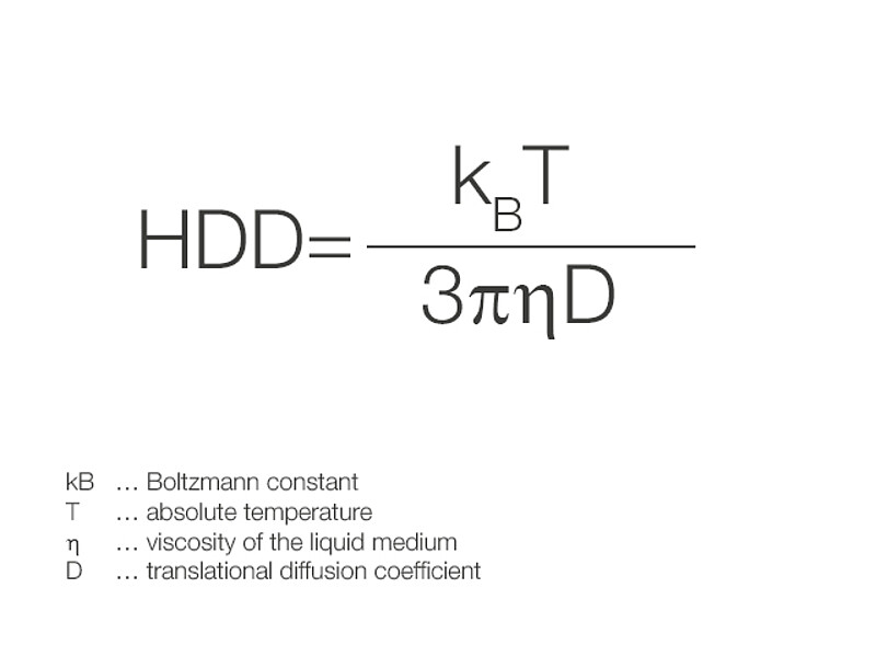
Dynamic light scattering (DLS), also called photon correlation spectroscopy (PCS), is an established and precise measurement method for characterizing particle size in suspensions and emulsions. It’s based on the Brownian motion of particles, which describes the random motion of particles suspended in a liquid or gas resulting from collision with other molecules in the surroundings. Smaller particles move faster, while larger ones move more slowly. With this technology, it’s possible to determine sizes from a few nanometers to the micrometer range). When the beam of a laser light hits the suspended particles, it’s scattered in all directions (Rayleigh scattering). The scattered light from different particles in the sample interferes and causes intensity fluctuations that are measured. They’re then converted to particle size and particle size distribution via the Stokes-Einstein equation, which assumes spherical particles.

The most important measurement results that can be obtained from a DLS measurement are:

The hydrodynamic diameter (HDD) is the diameter of a sphere, which diffuses with the same speed (translational diffusion coefficient D) as the particle in the same fluid under the same conditions
It’s defined via the Stokes-Einstein equation:

ISO-defined polydispersity index (PDI)
D-values (e.g., D₁₀, D₅₀, D₉₀)
Particle size distribution, which is usually intensity-based but can be converted to a volume- and number-based distribution

DLS devices on the market usually comply to ISO 22412, which makes DLS a suitable technique for highly regulated industries. The most important applications for DLS are characterization of proteins, polymers, micelles, and other submicron particles, which are suspended/dissolved in a medium. DLS is a fast method. Accurate and reliable results are achieved within a few minutes. It’s a calibration-free method, which doesn’t require as much knowledge about your sample as, for example, laser diffraction measurements.

One of the limitations of DLS measurements is variation in results due to changes in temperature, which lead to a change in the sample’s viscosity. Often, samples containing closely related particles (e.g., particles of similar sizes) are not resolved, and the presence of aggregates may affect measurements.

Dynamic image analysis

Dynamic image analysis is a method to determine the particle size distribution and particle shape of a sample by continuously photographing the silhouette of dispersed particles. In contrast to laser diffraction and DLS, particle shape and aggregation state can be determined by this measurement method. During a measurement, the sample constantly flows past a camera. The dispersed particles can move randomly, which means that the camera can view them from all sides and thus determine their actual shape and particle size. The instrument software then calculates all relevant parameters and results in order to describe the particle’s size and shape:

Particle size
Projection area
Aspect ratio
Feret diameter
Area equivalent diameter of particle
Convexity

The most accurate results are obtained in a size range of 1 µm to 1000 µm. Examples of particle size and shape analysis applications are the analysis of fractions of different samples (e.g., catalysts, granules, breakage studies, etc.), determination of particles’ angularity, or the prediction of flow and compacting behavior in dependence of particle size and shape. The ISO norm 13322-2:2006 describes image analysis methods, making it possible to use this method in highly regulated industries as well.

Dynamic image analysis is a fast measurement method, usually taking up to only five minutes. Not only particle size, but also shape parameters, such as aspect ratio or convexity, can be obtained. As for laser diffraction, a representative sample volume is required to obtain meaningful and accurate results. For this method, sampling errors are the main source of unreliable measurement results.

Sieving

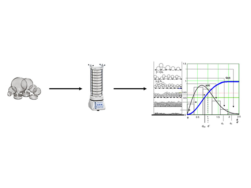
Sieving is the most traditional method to separate solid powders into defined fractions of specified particle size. Just like laser diffraction and dynamic light scattering, sieving relies on the assumption of spherical particles. The size classes, which are used to establish a particle size distribution, are defined by the chosen mesh size of the dedicated sieves. A powder is sieved through a stack of sieves with increasing mesh size for a defined period of time (e.g., 15 minutes). A shaker is used to vibrate the stack, which also causes non-spherical particles to reorient themselves to fit through the meshes of the sieve. After the separation process, the powder retained in each sieve is weighed and a cumulative mass-derived particle size distribution is calculated. Sieving enables the analysis of powders ranging in size from 20 µm to several centimeters.

Many different industries, especially the mining and building industry, still use sieving as the method of choice, and it’s often referred to as the reference method for other particle characterization techniques (e.g., laser diffraction).

Figure 2: Different sieves with different mesh sizes stacked on a shaker and the resulting particle size distribution.

Sieve analysis is a low-cost technique, which is widely accepted in many different industries mainly because of its robustness. It’s insensitive to dust, shaking, and heavy mechanical load. However, it’s time consuming to assemble and disassemble the sieves, which is a disadvantage of this method. Due to the distortion caused by anisotropy of the measured particles, the fine fraction is usually overrepresented. Today, since faster and more informative methods have been developed, the importance of sieve analysis has been decreasing.

Sedimentation analysis

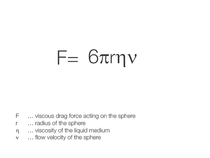
Sedimentation analysis is a method for determining the size of solid particles ranging from 1 μm to 100 μm. For particle size determination, Stokes’ law is used: A glass tube contains a stationary fluid (e.g., distilled water or organic solvents) in which a sphere (particle) with a known density descends through the liquid. The particle size can be calculated using Stokes’ law if the viscosity of the liquid, the particle’s density, and the velocity of the particle descending in the fluid are known:

Figure 3: Schematic illustration of sedimentation analysis.

Sedimentation analysis is commonly used in the soil industry or in geology to classify different sediments. The major advantage is that it doesn’t require a high investment. Sedimentation enables continuous operation, produces a high degree of accuracy and repeatability, and a relatively broad size range can be tested. However, gravitational sedimentation is usually limited to particles in the micrometer range, as the rate of sedimentation for small particles is too low to offer a user-friendly and practical analysis time. Moreover, Brownian motion of small particles would affect their settling movement too much to allow an effective measurement.

Nanoparticle tracking analysis

Nanoparticle tracking analysis (NTA) is a method to measure nanoparticles in the size range of 30 nm to 1000 nm. Like DLS measurements, this technique is based on Brownian Motion, which is measured to calculate the translational diffusion diameter and the hydrodynamic diameter.

Particles in suspension are illuminated by a laser beam, and the particles scatter light, which is detected by a camera (CCD or CMOS). This camera is set up at a specific angle to the sample (Figure 4). Particles are individually tracked, and their size is calculated by tracing their path. Usually, the resulting particle size distribution is number based.

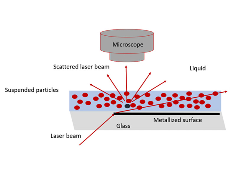
Figure 4: Schematic setup of NTA analysis.

NTA allows measurement not just of size but also of sample concentration via knowledge of the sample’s measurement volume. The measurement setup is standardized by the ASTM E2834-1 norm. The main applications of this method are characterization of dispersed nanoparticles, such as proteins, nanobubbles, or drug-delivery systems, to obtain insight in polydisperse samples. Nano-tracking analysis returns accurate measurement results for mono and polydisperse samples. However, NTA results are less reproducible and more time-consuming compared to other techniques such as DLS. Moreover, sample preparation is an important step and handling can impact the obtained size distribution. Therefore, experienced users are required. Moreover, NTA is a single particle method, which means that a limited number of individual particles is measured. This can cause measurement errors due to the fact that small particle fractions, for instance large aggregates, are overseen because their number in the sample is small.

Coulter measuring principle

Measurements with a Coulter counter device are based on the change of the mean electrical conductivity between two electrodes. These electrodes are immersed in an electrolyte solution containing particles with a different conductivity than the electrolyte. For particle counting, the device consists of two chambers (Figure 5). The electrodes are separated from each other by a narrow capillary, whose size depends on the particle size to be measured. The capillary’s diameter should be only slightly larger than the particles’ diameter. A pump creates negative pressure in one chamber, which then creates a flow from one chamber to the other. Particles moving from one chamber to the other result in a change of the resistance between the two electrodes – small particles lead to a smaller change, and larger particles will lead to a larger change of the signal. The user obtains the results on particle number and size via resistance changes from voltage pulses, which are plotted over time.

This method can be used to measure any particulate material that can be suspended in an electrolyte solution. Particles as small as 0.4 µm and as large as 1600 µm in diameter can routinely be measured.

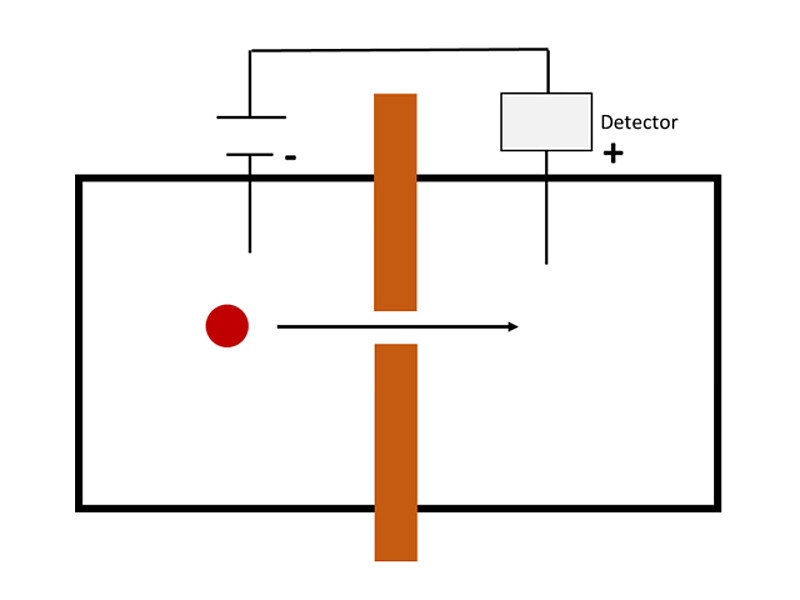
Figure 5: Schematic measurement setup of a Coulter counter device.

The Coulter method is widely used in medical and research labs (e.g., for cell counting or blood cell characterization). It’s also used for characterization of liposomes, exosomes or virus-like particles. This method is easy to apply and independent of optical and chemical properties of the particles. It can be used for any particles that can displace liquid. However, the size range is quite limited and apertures are easily blocked.

Summary

In this article, different methods for particle characterization were presented. Each technique has different advantages and disadvantages and is suitable for different types of samples and particulate matter of different sizes. Whereas classical sieve analysis can be used only for dry powders, dynamic light scattering, nano-tracking analysis, and sedimentation analysis require measurement of the sample in a liquid/dispersed state. Laser diffraction and dynamic image analysis allow measurement of the sample in liquid and dry states. In order to choose a suitable measurement device, these and other parameters need to be considered. Furthermore, to properly interpret the results the user must be aware of the limitations and inherent bias of the used technique.

Cross references

Particle size analysis methods: Dynamic light scattering vs. laser diffraction
Particle size distribution
Particle size determination for industrial applications
The principles of dynamic light scattering
Laser diffraction for particle sizing
How to choose an instrument for particle analysis

Bewerte diese Seite

You had already rated this article

Frequently viewed