Basis of Differential Scanning Calorimetry
This article provides an introduction to the principles and fundamentals of differential scanning calorimetry (DSC), a widely used thermal analysis technique essential for both traditional and modern methods of materials characterization. In celebration of the launch of our new Julia DSC 300 and 500 instruments, we invite you to explore the thermal insights – both “hot” and “cold” – that DSC can reveal about material behavior.
Differential Scanning Calorimetry (DSC)
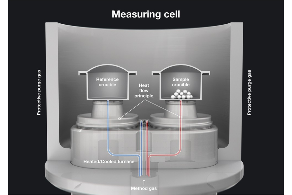
Differential scanning calorimetry (DSC) is a thermal analysis technique that measures the heat exchanged by a sample during a physical or chemical process. The term “differential” refers to the fact that the instrument measures the difference in heat flow between a sample and an inert reference. During analysis, the sample is heated up or cooled down within temperature ranges, thus the name “scanning.” DSC enables easy, reproducible analysis of thermal events and chemical induced changes in different materials. Practically, a small amount of sample is put in a crucible and measured together with an empty crucible of the same type, called the “reference.” The instrument determines how much energy is needed to heat up the sample compared to the reference over time. This energy is referred to as heat flow.
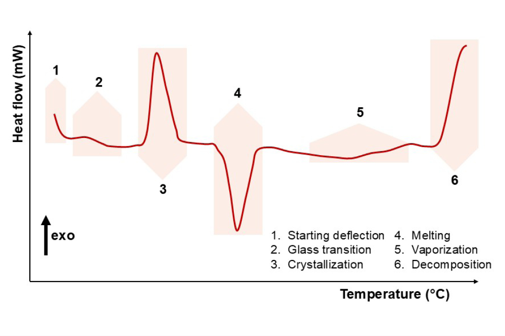
The analysis output of a DSC analysis, referred to as a thermogram, shows the transitions occurring in the selected temperature range. These transformations are usually either endothermic or exothermic processes. In short, the sample can absorb energy (an endothermic event) or release energy (an exothermic event). An example is the melting of a crystalline structure: breaking the order induced by a crystalline arrangement requires energy, making the transition endothermic. The crystallization of a material, however, is exothermic, as the molecules reach a higher ordered state and release energy. The thermogram will show different peaks, endothermic or exothermic, depending on the sample. From their shape, area, and position, we can then interpret the material’s history and characterize its thermal behavior.
While DSC is widely used in the polymer industry, it also offers valuable applications in the pharmaceutical, petrochemical, and food industries.
Thermal analysis techniques and their applications
Thermal analysis includes a range of different techniques, from thermal gravimetric analysis (TGA) to thermomechanical analysis (TMA) and dynamic mechanical analysis (DMA). The table below shows their possible applications.
Table 1
| Application | DSC | TGA | TMA | DMA | |
| Thermal properties | Specific heat capacity (cp) | + | |||
| Enthalpy changes, enthalpy of conversion | + | ||||
| Melting enthalpy, crystallinity | + | ||||
| Melting point, melting behavior (liquid fraction) | + | ||||
| Purity of crystalline organic compounds | + | + | |||
| Crystallization behaviour, supercooling | + | ||||
| Vaporization, sublimation, desorption | + | + | |||
| Solid-solid transitions, polymorphism | + | ± | |||
| Glass transition, amorphous softening | + | + | + | ||
| Thermal decomposition, pyrolysis, depolymerization, degradation | ± | + | ± | ||
| Temperature stability | ± | + | ± | ||
| Chemical properties | Chemical reactions | + | ± | ||
| Investigation of reaction kinetics and applied kinetics | + | + | |||
| Oxidative degradation, oxidation stability (OOT, OIT) | + | + | ± | ||
| Compositional analysis | + | + | |||
| Comparison of different batches and competitive products | + | + | ± | ± | |
| Mechanical properties | Linear expansion coefficient | + | |||
| Elastic modulus | ± | + | |||
| Shear modulus | + | ||||
| Mechanical damping | + | ||||
| Viscoelastic behaviour | ± | + |
+, very suitable; ±, less suitable
Of all the thermal analysis techniques, DSC offers the broadest applicability for characterizing both thermal and chemical properties.
What is differential scanning calorimetry?
The principles behind DSC
Differential scanning calorimetry (DSC) measures the difference in heat flow between a sample and an inert reference as they are heated or cooled. When the sample undergoes physical or chemical transitions – such as melting (endothermic) or crystallization (exothermic) – the heat flow changes, with these events appearing as peaks in the DSC signal.
Types of DSC
There are two types of DSC:
- Heat-flux
- Power compensated
Here we will focus on heat-flux DSC, since this is the technology underpinning the Julia DSC instruments. In a typical heat-flux DSC, sample and reference crucibles sit on separate sensors connected to thermocouples inside a temperature-controlled furnace. The temperature difference between the two sensors is proportional to the heat flow needed to maintain identical heating conditions. The heat flow is directly related to both the enthalpy changes occurring in the material and the heat capacity. By tracking heat flow as a function of temperature, DSC can characterize thermal transitions and, with appropriate calibration, determine quantities such as heat capacity (Cp) and transition enthalpies.
In a power compensated DSC, the sample and reference crucibles are housed in separate furnaces, allowing for independent temperature control. The primary measured value is the electrical heating power needed to keep the sample and reference temperatures as close as possible. Because electrical power is the registered signal, this type of DSC can achieve very high cooling and heating rates while requiring only small sample quantities.
Typical thermal transitions
For the correct interpretation of a thermogram, it is important to indicate the direction of exothermic events. Exothermic events typically point up (indicated by an arrow). Below, we illustrate the most common thermal events that can be observed during a thermal analysis, plotted at progressively increasing temperatures.
Introducing Julia DSC
Anton Paar offers two heat-flux DSC models: Julia DSC 300 and 500. Coupled with our Julia Suite software, they are suitable for applications ranging from research to quality control across a vast range of materials. Depending on the cooling module, the temperature range spans from as low as -170 °C to 700 °C. The removable trays accommodate 70 samples, with a dedicated space for up to eight different references. Both devices can be equipped with an autosampler for 24/7 unattended operation.
Differences between Julia DSC 300 and DSC 500
Julia DSC 300 supports the Air Cooling Module, covering a temperature range of -35 °C to 700 °C. Julia DSC 500, on the other hand, is compatible with all of our available cooling modules, reaching a minimum temperature of -170 °C. Both models can be equipped with an autosampler for reduced operational workload.
Cooling module selection
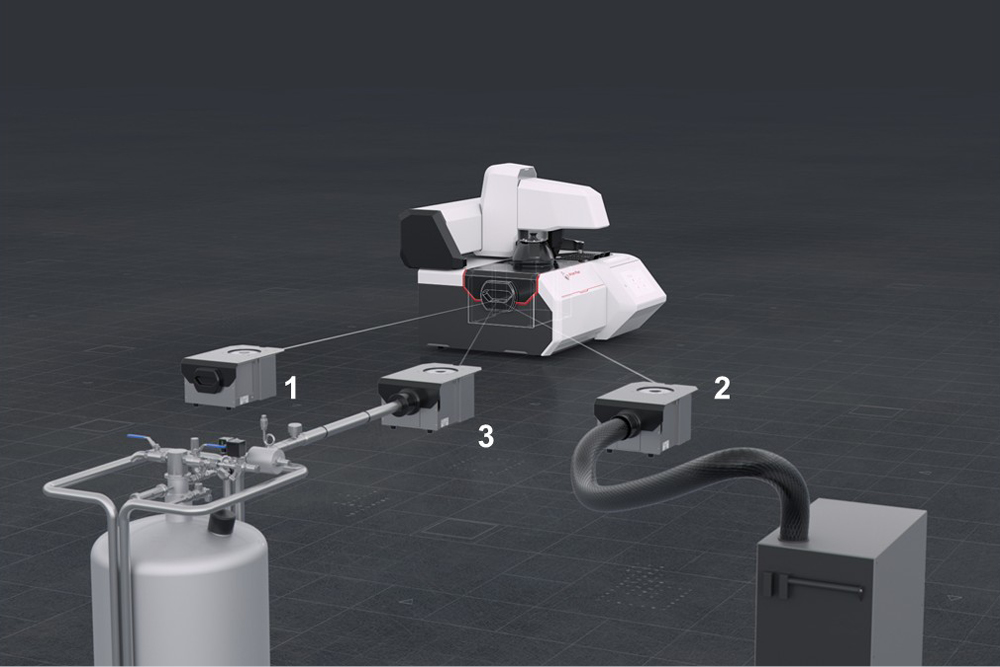
Air Cooling Module (ACM)
Our patented Peltier built-in air-cooling module reaches sub-ambient temperatures down to -35 °C. The ACM supports a maximum temperature of 700 °C, with a maximum heating rate of 300 K/min and a maximum cooling rate of 150 K/min.
Refrigerated Cooling Module (RCM)
The RCM reaches temperatures of -90 °C, with a maximum cooling rate of 150 K/min. The maximum temperature is 700 °C, with a maximum heating rate of 300 K/min. Its closed-circuit design eliminates the need for the user to refill the coolant. The RCM is well-suited to exploring lower temperature transitions, such as those typical of polymers. It is compatible with Julia DSC 500 only and requires additional space beside the instrument.
Nitrogen Cooling Module (NCM)
The NCM is designed for analysis across a complete temperature range, from -170 °C to 600 °C. It offers a maximum heating rate of 300 K/min and a maximum cooling rate of 200 K/min. This powerful cooling module is ideal for reaching the lowest temperatures, making it especially valuable for research on specialized materials and low-temperature transitions. The NCM requires additional space beside the instrument for the nitrogen dewar, which needs periodic filling. It is compatible with Julia DSC 500 only.
Calibration
Calibration is fundamental to obtain true values from a measurement. As heat-flux DSC is based on an indirect measurement of the sample temperature – rather than the actual temperature – the values can deviate from the true ones depending on the setup. Measuring known standards establishes a relationship between the displayed values and the real (literature) values of thermal properties. Indium is typically used for this purpose, with a melting point of 156,60 °C and a fusion enthalpy of 28,58 J/g. The scaling factors determined during calibration are used to adjust the measured values accordingly.
For a calibration performed with Julia DSC 300 and 500, at least two calibrants are needed to calculate the correction within the temperature range between them. Indium and zinc (melting point: 419,53 °C) are commonly used to calibrate measurements between 120 °C to 470 °C. It is also useful to perform sub-ambient calibrations. Common calibrants for this task include water (0.0 °C), n-dodecane (-9.65 °C), and n-octane (-56.85 °C). Calibrants should be selected according to the cooling module used and the analysis type. The following table lists the characteristic values and recommended sample masses for the most commonly used calibrants.
Table 2
| Calibrant | Tmelting (°C) | Enthalpy (J/g) | Mass (mg) |
| Indium (In) | 156.6 | 28.58 | 7.5-11 |
| Zinc (Zn) | 419.53 | 111.99 | 1.8-2.8 |
| Tin (Sn) | 231.96 | 60.48 | 3.5-5.3 |
| Water | 0.0 | 334.16 | 0.6-1.0 |
| n-dodecane | -9.65 | 216.16 | 1.0-1.5 |
| n-octane | -56.85 | 181.57 | 1.1-1.8 |
During calibration, it is also possible to calibrate the temperature modulation for sinusoidal DSC or SDSC. SDSC is used to separate the contributions of reversible and irreversible thermal events during analysis. Melting, crystallization, and glass transition are considered reversible, whereas enthalpy relaxations superimpose on the glass transition are irreversible. Calibration for SDSC should be performed at two different heating rates, typically between 5 K/min and 20 K/min.
As the compensation terms depend on the crucible type, the crucible’s contribution should also be included. This is done during TruPeak measurement. Due to the intrinsic differences between sensors, asymmetries in the instrument can introduce systematic errors. TruPeak involves a series of calibration measurements using sapphire – chosen for its heat capacity – as well as with empty furnaces and crucibles to determine a good baseline for future analysis.
Preparing and conducting a DSC measurement
Toolbox
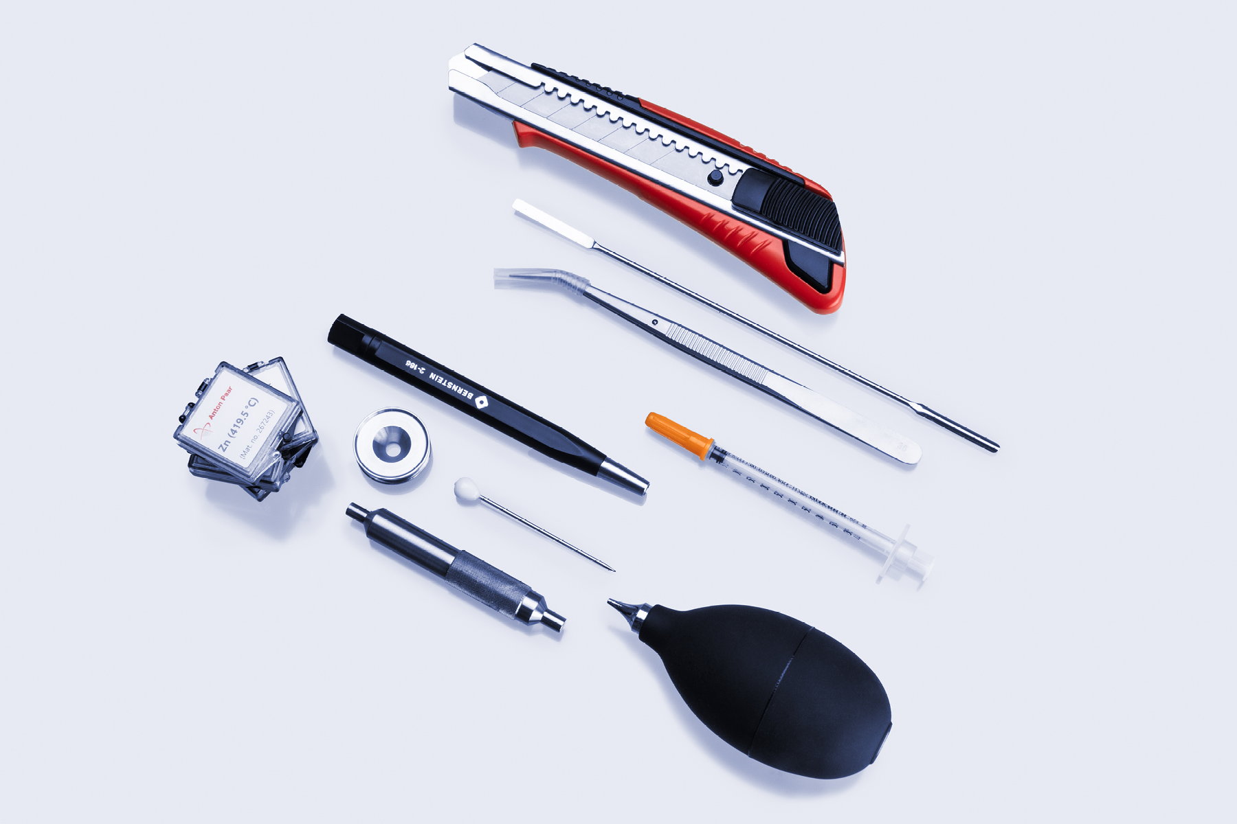
Each Julia DSC is equipped with a sample preparation toolbox that includes everything from a blade and syringe to a push rod and funnel. Cleaning tools for the furnace are also provided, such as a glass fiber brush for the sensors and a blowing bell for the furnace cell.
Crucibles
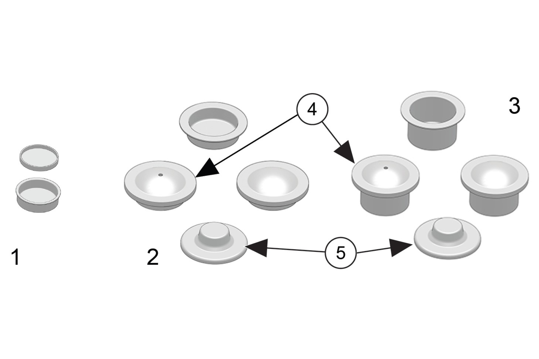
In principle, any type of crucible can be used with the Julia DSC instruments after proper calibration. However, Anton Paar provides a range of benchmarked crucibles optimized for everyday analysis and categorized by size and suggested application. We recommend not to fill crucibles beyond two-thirds capacity to prevent contamination of the rims and sample spillage.
- Aluminum (Al) 20 µl crucible – closed or open (pan only)
Ideal for small quantities of sample (solids, powders), this crucible is not compatible with the sealing press. The lid, which is not hermetically sealed, is closed using a push rod. This makes the crucible especially well-suited for foils or fibers, as the lid ensures better thermal contact between the samples and the crucible bottom, leading to more accurate results. - Aluminum (Al) 40 µl crucible – closed or open (pan only)
The most commonly used crucible, this is suitable for a wide range of sample types, including liquids when used with the full lid. It can be hermetically sealed using the sealing press. The lid is cold welded to the crucible. - Aluminum (Al) 100 µl crucible – closed or open (pan only)
Used when larger amounts of sample are required, this crucible is compatible with any kind of sample. It can be sealed using the sealing press. - Pre-pierced lids – for both 40 and 100 µl crucibles
Pre-pierced lids feature a laser-cut hole in the same diameter and position. This is the most common lid used in experiments as it prevents the crucible from popping due to the buildup of internal pressure during analysis. Pre-pierced lids are also suitable for solid compounds. - Pierceable lids – for 40 and 100 µl crucibles (only for use with Autosampler)
Pierceable lids are designed to be used exclusively with the Autosampler. They are ideal for samples that need to be treated in an inert or controlled atmosphere until the moment of measurement (e.g., reactive compounds). The Autosampler is equipped with a software-controlled needle, which pierces the lid directly in the furnace just before the measurement begins.
Standard full lids (used with 40 and 100 µl crucibles) can be manually pierced using a needle, such as the one provided in the toolbox. Piercing the lid before performing a DSC measurement allows developed vapors to escape, preventing deformation of the crucible. Crucible pans may also be used without a lid for special applications such as oxidation analysis or when a reaction between the sample and a method gas is required.
Note: Always wear gloves and protective glasses when handling samples!
Samples
Powders
Powdered samples often contain a large amount of air, which is a poor thermal conductor. For optimal thermal contact, it is good practice to compact the powder firmly in the crucible using the push rod, always pressing against a hard surface to avoid deforming the crucible bottom. This improves contact between the sample and the crucible bottom. To prevent contamination of the crucible rim during filling, a funnel is recommended. A pre-pierced lid is typically used for standard analyses. Powders can also be loaded in the crucible pan without a lid for oxidative studies.
Step-by-step guide:
- Weigh the empty crucible and lid (if required)
- Load the powder using a spatula and funnel
- Compact the powder using the push rod
- Seal the crucible (if required) with the appropriate lid using the sealing press
- Weigh the filled crucible and determine the sample mass by difference
Note: If using an Al 20 µl crucible, close the lid using the push rod
Liquid samples
The wetting behavior and volatility of liquid samples should be carefully considered during sample preparation. Only 40 and 100 µL aluminum crucibles with hermetically sealed lids are recommended for such samples. This prevents sample loss before and during the analysis, as mass losses greater than 1 % can significantly impact DSC results. Low-temperature calibrants, which are often liquid at room temperature, are typical examples of liquid samples that require special care during preparation.
Step-by-step guide:
- Weigh empty crucible and lid
- Load the liquid sample using the syringe from the toolbox
- Deposit a small amount in the crucible paying attention not to spill it on the rim
- Seal the crucible and weigh
- Determine the sample mass by difference
Foils and fibers
Achieving the best possible thermal contact to the bottom of the crucible is crucial for the analysis. Fibers and foils are light and can possibly bend and tilt if the crucible used is too big (40 or 100 µl crucibles). We suggest using the 20 µl crucibles with a lid, which is pressed down onto the sample during the analysis. This will also improve the baseline.
Step-by-step guide:
- Weigh empty crucible and lid
- Load the sample using the tweezers from the toolbox
- Press the lid onto the crucible using the correct side of the push rod
- Weigh the filled crucible and determine the sample mass by difference
Creating a temperature method
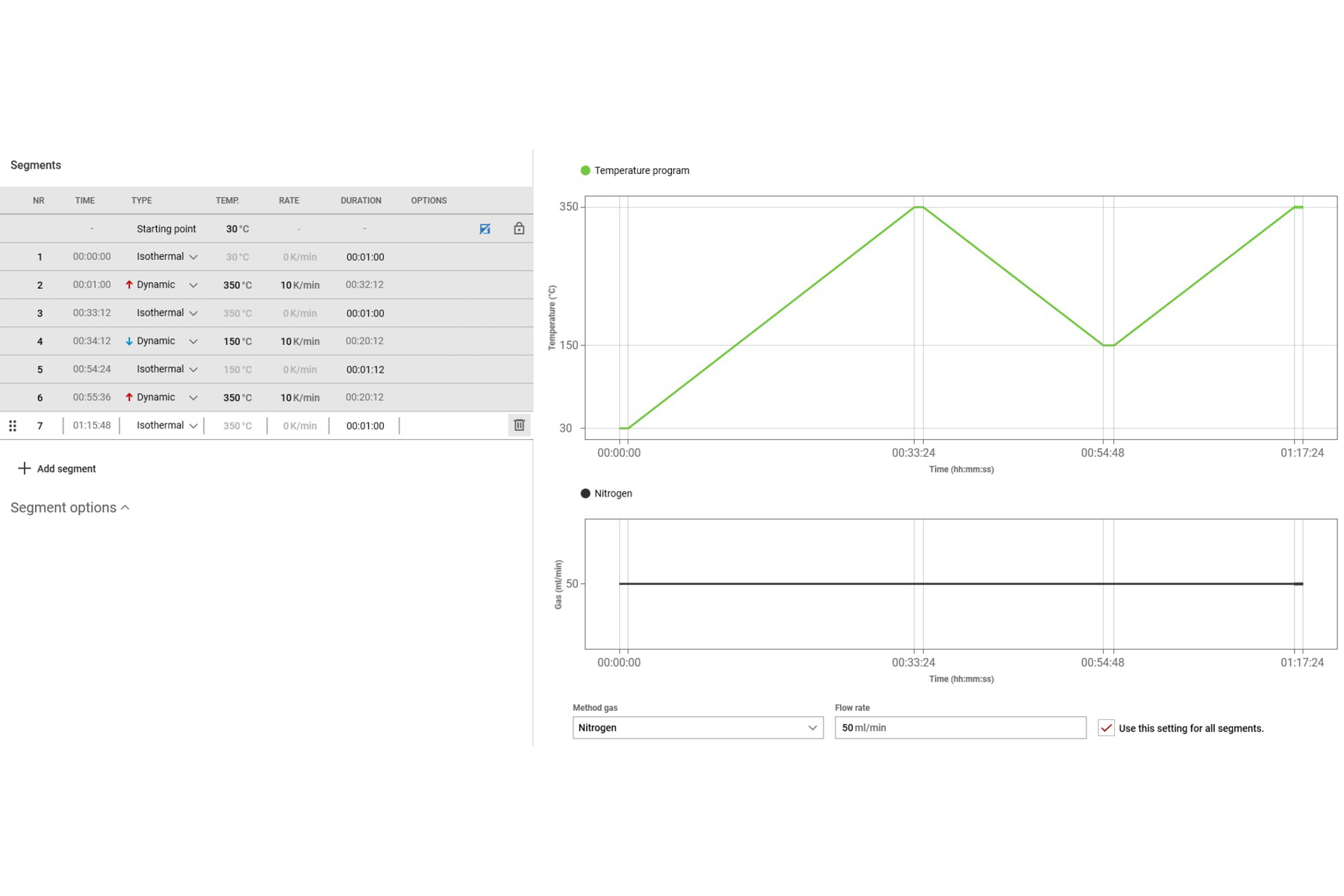
Creating a method is a fundamental step in preparing for a DSC analysis. While knowledge of the sample is helpful, a well-defined method can make the difference between a good measurement and a bad one. With Julia Suite, temperature methods can be created intuitively by selecting from various segments and purging gases. (Note: The temperature limits will depend on the type of cooling module used.)
Method development involves setting the temperature, heating and cooling rates, method gases, and the type of analysis to be performed. Below are some key considerations to keep in mind when preparing a method.
- It is important to set a starting temperature two to three minutes before the beginning of the first expected transition, taking into account the selected heating rate. This corresponds to around 20 °C before the transition when using a heating rate of 10 K/min.
- A heating rate that allows clear observation of the transition without losing information is preferrable. Standard heating rates are between 5 K/min to 20 K/min. Increasing the heating rate enhances the sensitivity of the instrument (stronger signal). However, this comes at the cost of resolution. To improve resolution, lower heating rates are preferred.
- The end of the analysis should be set two to three minutes after the end of the transition, which corresponds to 20 °C beyond the expected transition temperature at a heating rate of 10 K/min.
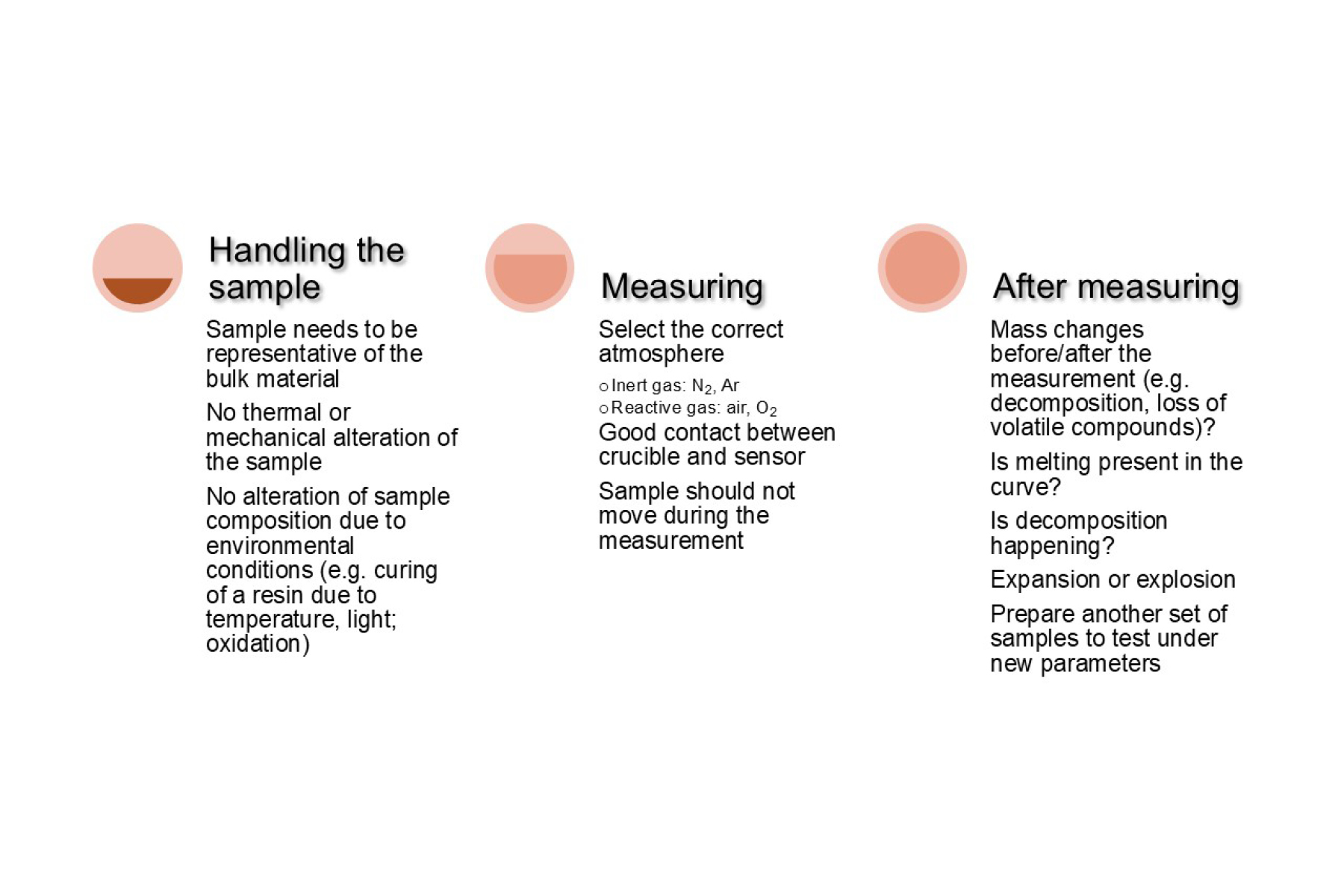
- The method gas should be selected according to the type of analysis. For oxidation or decomposition, a reactive gas such as air or oxygen is used. In other cases, inert gases such as nitrogen, argon, are preferred. OIT (oxidation induction time) and OOT (oxidation onset temperature) are typical examples where air or oxygen are required.
Typical segment types available in Julia Suite include:
- Isothermal: Maintains the temperature stable at an arbitrary value over an amount of time defined by the user
- Dynamic: Heats or cools the sample within a temperature range at a specific heating or cooling rate
- Ballistic: Heats the sample to a target temperature using the maximum heating rate
- Equilibrate: Heats the sample to a target temperature at the maximum heating rate and maintains it for 30 seconds
- Loop: Repeats a segment, changing the temperature extremes by a defined amount
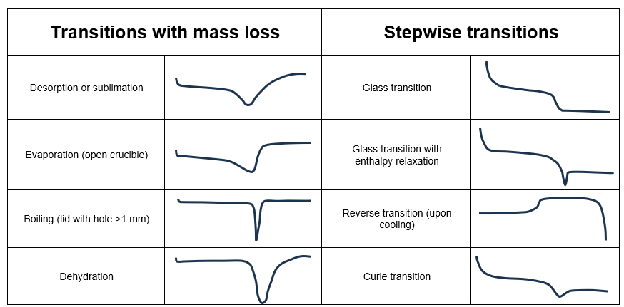
Understanding thermal events
The tables below can help users identify the transitions that characterize a sample. While glass transitions, melting, and crystallization points are the most common transitions observed during DSC analysis, there are many more depending on the type of sample and experimental conditions.
Table 3
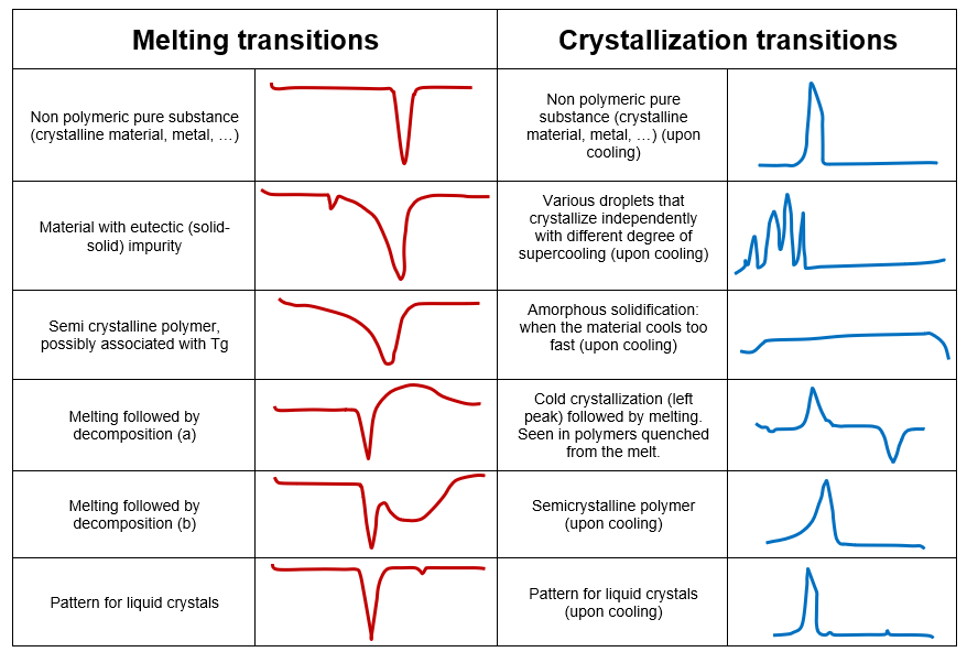
Table 4
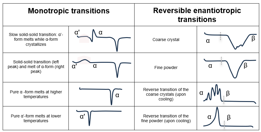
Table 5
Thermogram analysis
Julia Suite Professional provides a range of tools for analyzing thermograms, including peak analysis, the identification and calculation of the glass transition, and OIT/OOT determination. Selecting the appropriate baseline is essential for obtaining meaningful data. Likewise, selecting the correct transition ensures true values for the analyzed compound. Julia Suite Professional also offers different analysis options, including mathematical operations such as averaging and subtracting, to support optimal understanding of results.
Real-life applications
You can find our application reports here: www.anton-paar.com/at-de/produkte/details/julia-dsc/
We continue to research new applications for our devices, and we’re always open to fresh, interesting ideas. If you have an application you’d like to discuss, please reach out to our team at Application-Tan[at]anton-paar.com.
Relevant standards
- ASTM D3418 | Standard Test Method for Transition Temperatures and Enthalpies of Fusion and Crystallization of Polymers by Differential Scanning Calorimetry
- ASTM D3895 | Standard Test Method for Oxidative-Induction Time of Polyolefins by Differential Scanning Calorimetry
- ASTM D4591 | Standard Test Method for Determining Temperatures and Heats of Transitions of Fluoropolymers by Differential Scanning Calorimetry
- ASTM D6604 | Standard Practice for Glass Transition Temperatures of Hydrocarbon Resins by Differential Scanning Calorimetry
- ASTM E487 | Standard Test Methods for Constant-Temperature Stability of Chemical Materials
- ASTM E537 | Standard Test Method for Thermal Stability of Chemicals by Differential Scanning Calorimetry
- ASTM E793 | Standard Test Method for Enthalpies of Fusion and Crystallization by Differential Scanning Calorimetry
- ASTM E794 | Standard Test Method for Melting and Crystallization Temperatures by Thermal Analysis
- ASTM E928 | Standard Test Method for Purity by Differential Scanning Calorimetry
- ASTM E1269 | Standard Test Method for Determining Specific Heat Capacity by Differential Scanning Calorimetry
- ASTM E1858 | Standard Test Methods for Determining Oxidation Induction Time of Hydrocarbons by Differential Scanning Calorimetry
- ASTM E2009 | Standard Test Methods for Oxidation Onset Temperature of Hydrocarbons by Differential Scanning Calorimetry
- ASTM E2602 | Standard Test Methods for Assignment of the Glass Transition Temperature by Modulated Temperature Differential Scanning Calorimetry
- ASTM E2716 | Standard Test Method for Determining Specific Heat Capacity by Modulated Temperature Differential Scanning Calorimetry
- ISO 11357 | Plastics – Differential scanning calorimetry (DSC)
- ISO 19935 | Plastics – Temperature modulated DSC
- ISO 22768 | Raw rubber and rubber latex – Determination of the glass transition temperature by differential scanning calorimetry (DSC)
- DIN 51007 | Thermal analysis - Differential thermal analysis (DTA) and differential scanning calorimetry (DSC) - General Principles
- DIN 53545 | Testing of rubber - Determination of low-temperature behaviour of elastomers - Principles and test methods
- USP United States Pharmacopeia, section 891 | Thermal Analysis
- Ph. Eur. European Pharmacopoeia, section 2.2.34. | Thermal analysi
- JP Japanese Pharmacopoeia, section 2.52 | Thermal Analysis
References
Atkins, Peter, and Julio de Paula. Physical Chemistry. 9th ed., W. H. Freeman, 2009.
Billmeyer, Fred W., Jr. Textbook of Polymer Science. 3rd ed., Wiley-Interscience, 1984.
Ehrenstein, Gottfried W., et al. Praxis der Thermischen Analyse von Kunststoffen. 2nd ed., Fester Einband , 2003.
Frick, Achim, and Claudia Stern. DSC-Prüfung in der Anwendung. Carl Hanser Verlag GmbH & Co. KG, 2013.
Gabbott, Paul. Principles and Applications of Thermal Analysis. Blackwell Publishing Ltd, 2008.
Gaisford, Simon, et al. Principles of Thermal Analysis and Calorimetry. 2nd ed., RSC Publishing, 2016.
Groenewoud, W. M. Characterization of Polymers by Thermal Analysis. Elsevier Science B.V., 2001.
Höhne, Günter W. H., et al. Differential Scanning Calorimetry. 2nd ed., Springer, 2003.
Menczel, Joseph D., and R. Bruce Prime. Thermal Analysis of Polymers: Fundamentals and Applications. John Wiley & Sons, 2009.
Saadatkhah, Nooshin, et al. “Experimental Methods in Chemical Engineering: Thermogravimetric Analysis—TGA.” The Canadian Journal of Chemical Engineering, vol. 98, no. 1, 2020, pp. 34–43, doi.org/10.1002/cjce.23673.
Schick, C. “Differential Scanning Calorimetry (DSC) of Semicrystalline Polymers.” Analytical and Bioanalytical Chemistry, vol. 395, no. 6, 2009, pp. 1589–1611, doi.org/10.1007/s00216-009-3169-y.
Turi, Edith A. Thermal Characterization of Polymeric Materials. Academic Press, 2012.
Wagner, Matthias. Thermal Analysis in Practice: Collected Applications. 2nd ed., Mettler-Toledo GmbH, 2017.