Yield point, evaluation using the flow curve
Yield-point measurements are always comparisons of the acting forces: the internal cohesion force of the sample’s network of forces on the one side; and the external force acting upon the sample on the other side. Therefore, tests with preset force or controlled shear stress (CSS) will often deliver better results than tests with controlled shear rate (CSR).
From the rheological point of view, the yield point is a shear stress limit; its unit is Pa (pascal). The yield value determined by whatever means is not a material constant because it depends on the sample’s pretreatment and on the measuring method used, as well as on the evaluation method used.
Determination of the yield point using a flow-curve diagram
Method 1
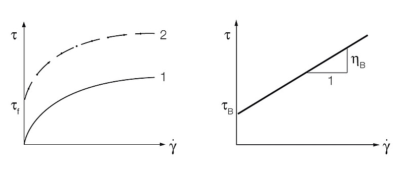
Determination of the yield point via the shear-stress-axis intercept of a flow curve: With this evaluation method, the measured flow curve is presented on a linear scale. Next, the yield point is read as the value on the shear-stress axis that appears at the beginning of the flow curve (Figure 1 left). This very easy method should only be used for simple quality assurance tests. Due to limited accuracy in the range of lower shear rates, this method is not recommended for tests in research and development.
Method 2
Determination of the yield point via mathematical curve-fitting models for flow curves: Flow curves consist of many individual measuring points. With this method, the yield point is evaluated by calculating a curve fitting that aims at the best possible superposition with the measured flow-curve values. The result is stated as a mathematical function. The three following model functions are commonly used. However, they are only suitable for simple quality control tests. Due to limited accuracy in the range of lower shear rates, they are not recommended for tests in research and development. In addition, there is a wealth of fitting models available.
Curve-fitting model according to Bingham
τ = τB + ηB ⋅ γ̇ with the Bingham yield point τB as an axis intercept and the Bingham viscosity ηB whose value is derived from the slope of the curve. This very simple model function plotted on a linear-scale flow-curve diagram shows a straight line with an intercept on the shear stress axis (Figure 1 right). Only the two evaluation parameters mentioned above are stated. In the lower shear-rate range, curve fitting is often rather imprecise.
Curve-fitting model according to Casson
The two fitting values here are the Casson yield point as the axis intercept and the Casson viscosity. Curve fitting is performed using the square-root function. The flow curve diagram on a linear scale shows that the model function is shaped as a curve with an intercept on the shear-stress axis (comparable with curve 2 in Figure 1 left). By taking the bend of the curve in the range of lower shear rates into consideration, this curve fitting model is often better than the Bingham model.
Curve-fitting model according to Herschel/Bulkley
In this model, the two parameters are the Herschel/Bulkley yield point as an axis intercept and the parameter p. Here again, the flow curve diagram on a linear scale shows that the model function is shaped as a curve with an intercept on the shear stress axis (comparable with curve 2 in Figure 1 left). The parameter p is used to differentiate within the flow range between shear-thinning (p < 1), shear-thickening (p > 1), and Bingham flow behavior (p = 1). Using these evaluation parameters, in most cases a better curve fitting will be achieved than with the Bingham model.
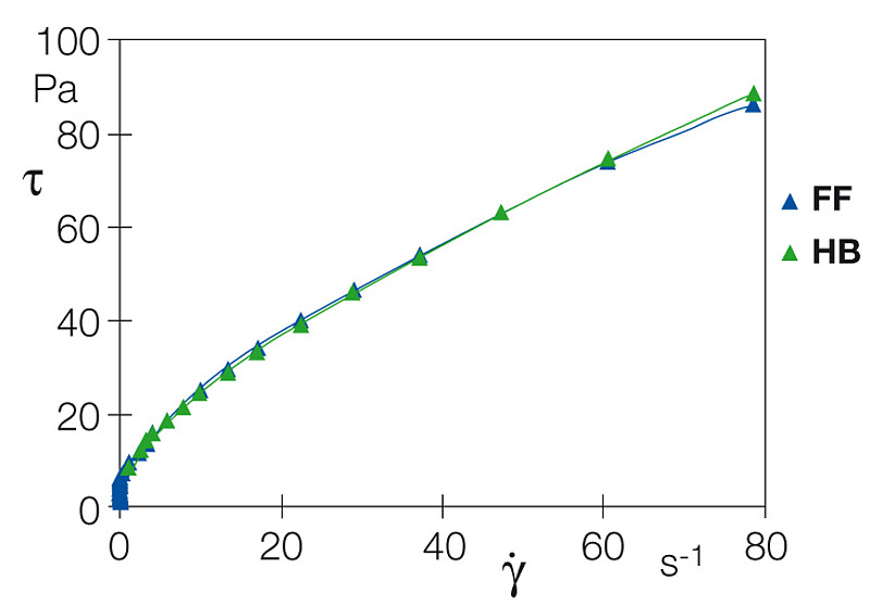
Measuring example:
Flow curve of a fracturing fluid and evaluation according to Herschel/Bulkley (Figure 2). Determination of the flow curve of a fracturing fluid using a special pressure cell at a pressure of 3 MPa (30 bar). Such fluids are used for the production of natural gas and crude oil. Using analysis software, the model function according to Herschel/Bulkley (HB) was calculated, resulting in a yield point of 5.9 Pa.
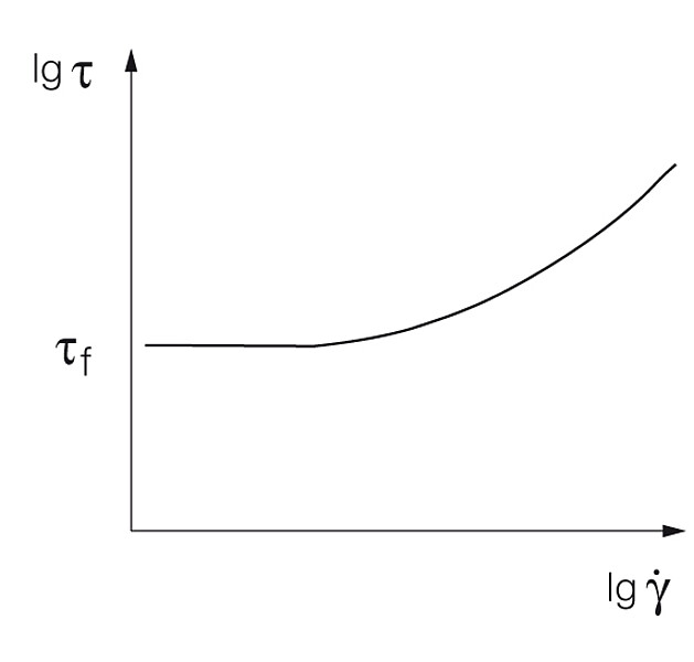
Method 3
Reading the yield point as the shear-stress value at the lowest shear rate (Figure 3)
Method 4
Reading the yield point at a previously set, very low shear rate: Here the shear rate, for example 1 s-1 or 0.1 s-1, is used for evaluation. Often scientists will even select a value of 0.01 s-1 to approximate the state at rest.