Instrumented indentation testing (IIT)
Hardness can be defined as the ability of a material to resist plastic deformation. This considerable property has been occupying metallurgists for decades, notably with the development of testing methods enabling them to measure and put values on that resistance. Although classical hardness testing such as Vickers, Brinell, or Rockwell testing has been widely used and improved throughout the 20th century, critical limitations have been revealed by the rise of micro- and nano-technologies.
History of indentation testing
Throughout the 20th century, the main classical hardness testing methods – Brinell, Vickers, Rockwell, and Knoop – were improved and defined as standards. However, the drawbacks of these techniques remained, especially when it came to characterizing coatings and thin films.
With the progress of miniaturization, alternative methods have been developed to characterize mechanical properties down to the nanometer scale. In 1992, Warren Oliver and George Pharr published an article on Instrumented Indentation Testing (IIT), also known as Depth Sensing Indentation (DSI), in which they described a methodology for measuring material hardness and elastic modulus by instrumented indentation. Unlike classical hardness testing, this quasi-static indentation method is achieved by pressing an indenter, usually a diamond of known geometry, into the surface to be tested with an incremental load. During that indentation, both indentation depth and normal load are monitored all along the insertion and withdrawal of the indenter. This results in the drawing of a loading and unloading curve of the applied load as a function of the indentation depth.
Advantages of instrumented indentation testing
Unlike conventional testing, IIT can be applied on thick to thin coatings and on bulk from hard to soft materials.
One of the major advantages of instrumented indentation testing (IIT) is also that, by means of a series of mathematical equations, an instrumented hardness (HIT) and an instrumented elastic modulus (EIT) are calculated in a single fast measurement. Observation and measurement of the residual print are no longer required. Measurements can therefore be fully automated with the definition of matrices or specific measurement protocols. Today, new analysis methods have been implemented that enable the determination of additional properties of a tested material, such as, among others, creep behavior and viscoelastic properties.
IIT is therefore a very versatile technique that is suitable for research and development work as well as quality control.
Principle of instrumented indentation testers
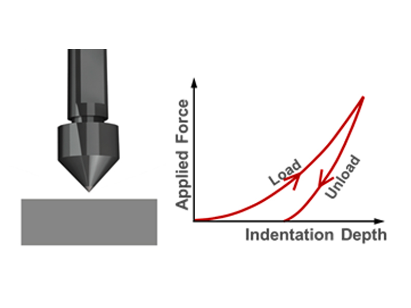
Instrumented indentation testers use a well-established method in which an indenter tip with a known geometry is driven into a specific area of the material to be tested by applying an increasing normal load. The indentation depth is monitored throughout the experiment by means of a displacement sensor.
For each loading-unloading cycle, the applied load value is plotted with respect to the corresponding position of the indenter. The resulting load vs. indentation depth curves provide data specific to the mechanical nature of the material under examination. Established models are used to calculate quantitative hardness and elastic modulus values for such data.
The ISO 14577 standard specifies that the method of instrumented indentation testing can be load-controlled or depth-controlled for the determination of the mechanical properties of materials. It also defines three ranges of measurement:
Indentation range
| Macro range | 2 N ≤ F ≤ 30 kN |
| Micro range | F < 2 N; h > 0.2 µm |
| Nano range | h ≤ 0.2 µm |
Analysis of the loading-unloading curve
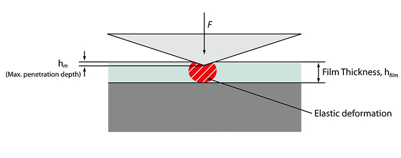
The indenter, initially in contact with the surface, is driven into the material at a predefined velocity until it reaches a preset load or a maximum preset depth. The load is then decreased down to zero with the same speed (unloading). In the case of a thin film, it should be noted that in order to avoid the effect of the substrate on the measured hardness and elastic modulus, the maximum indentation depth of the indenter should not exceed 10 % of the thin film thickness.
The following figure shows the response of an elastic-plastic material during the indentation by a Berkovich tip. In this figure, hc, which is the contact depth, is defined as the indentation depth when the indenter is in contact with the sample.
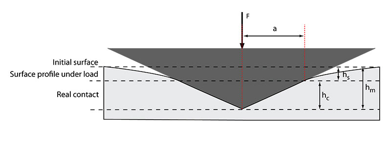
During the test, h, which is the depth measured, can be described by the following relation:
$$h_m = h_s + h_c$$
Equation 1
hs is the displacement of the surface at the perimeter of the contact and hc is the vertical distance along which contact is made. At peak load, the load and displacement are Fm and hm, respectively, and the radius of the contact is a.
The contact depth hc is calculated according to ISO 14577 using the following equation:
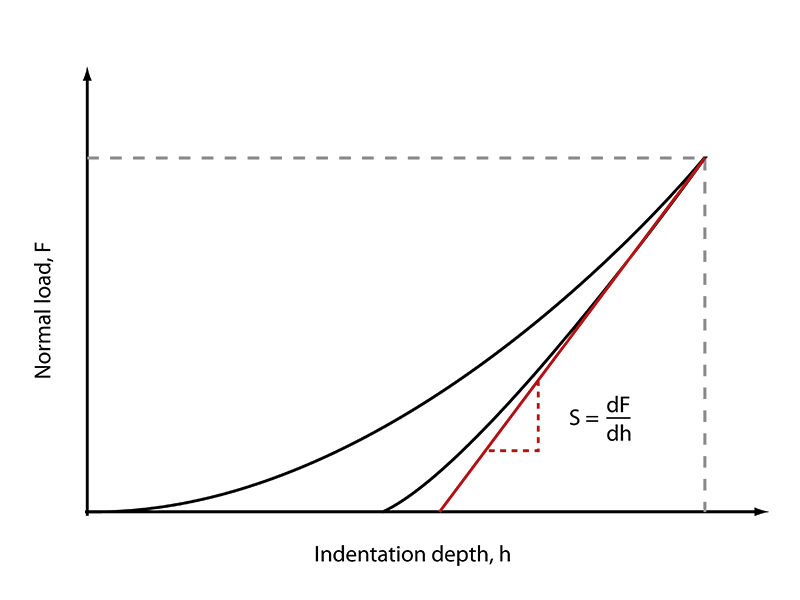
$$h_c = h_m - \varepsilon \frac{F_m}{{S}}$$
Equation 2
Where hm is the maximum indentation depth, Fm the maximum normal load, ε is a constant related to the indenter geometry and S is the sample’s stiffness calculated from the unloading portion of the indentation curve.
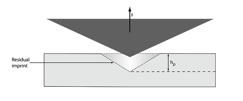
When the indenter is completely withdrawn and elastic displacement recovered, the final depth of the residual hardness impression is hp.
Thickness influence
One of the most popular applications of nanoindentation is the determination of the mechanical properties of thin films. However, the main difficulty encountered in the nanoindentation of thin films is to avoid the influence of the substrate.
The common approach for isolating the film properties of the substrate is to adopt an often-used guideline which consists in making measurements to a maximum indentation depth of no more than 10 % of the film thickness. More advanced methods have also been published but they generally require more complex testing such as dynamic indentation and/or proprietary software (Siomec, etc.).
Instrumented hardness calculation
The hardness is expressed by the ratio between the applied load and the contact area. In practice:
$$H_{IT} = \frac{F_m}{A_p}$$
Equation 3
Fm is the maximum load and Ap is the contact area between the indenter and the specimen at the maximum depth and load.
Instrumented elastic modulus calculation
As described in the ISO14577 standard, the reduced modulus, Er, is used to account for the fact that the elastic displacements occur in both the indenter and the sample. The instrumented elastic modulus in the test material, EIT, can be calculated from Er using the following formula:
$$\frac{1}{E_r}= \frac{(1-{\nu_s}^2)}{E_{IT}} + \frac{(1-{\nu_i}^2)}{E_{i}} $$
Equation 4
νs is the Poisson’s ratio for the sample and Ei and νi are the elastic modulus and Poisson’s ratio, respectively, of the indenter.
This reduced elastic modulus can be linked to the measured stiffness S by the relation:
$$E_r = \frac{\sqrt{\pi}}{2\beta}\frac{S}{\sqrt{A_p}}$$
Equation 5
The instrumented elastic modulus of the measured sample can then be calculated thanks to the equation below:
$$E_{IT} = \frac{(1-{\nu}^2)}{\frac{1}{E_r} - \frac{(1-{\nu_i}^2)}{E_i}}$$
Equation 6
The indentation modulus EIT is comparable with the Young’s modulus of the material.
When the Poisson’s ratio of the sample is unknown, a plane strain modulus can also be calculated.
$$E^{\ast} = \frac{1}{\frac{1}{E_r} - \frac{1-({\nu_i}^2)}{E_i}} = \frac{E_{IT}}{1-({\nu_s}^2)}$$
Equation 7
Determination of the projected contact area (Ap)
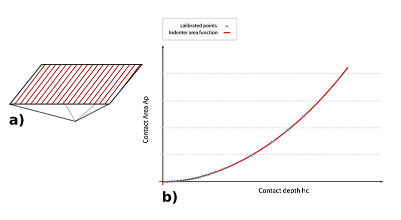
As shown above, the calculation of HIT and EIT is influenced by the indenter area function Ap.
For an ideally sharp indenter, the area function is:
$$A_p = {C_0}{h_c}^2$$
Equation 8
hc is the contact depth (see Figure 3).
This equation can be used to provide a first estimate of the contact area, where the constant C0 depends on the indenter geometry (C0=24.5 for a Berkovich and 6.3 for a cube-corner indenter).
However, indentation tips never have the ideal (theoretical) shape, which has to be taken into consideration, especially when indenting at shallow depths, by calibrating the indenter area function. The ISO standard 14577 describes two methods for determining the full tip area function:
- direct measurement using a traceable atomic force microscope (AFM)
- indirectly by running indentation measurements into a material of known Young’s modulus (or known plane strain modulus) and Poisson’s ratio.
Even if the first method gives accurate results, the indirect method is the most widely used because of the ease of implementation. Experimentally, multiple indentations are made under incremental loads on a material of certified properties (usually fused silica). For each measurement, the stiffness S and contact depth hc are calculated and the projected area calculated according to Eq. 5 explained above.
The evolution of Ap versus contact depth can then be fitted and plotted thanks to the following fitting function:
$$A_p = {C_0}{h_c}^2 +{C_1}{h_c} +{C_2}{h_c}^{\frac{1}{2}}+ ...+ {C_8}{h_c}^{\frac{1}{128}}$$
Equation 9
The constants C0…C8 can be determined by data measurement and the method outlined by Oliver and Pharr. This full tip function is necessary if accurate values of EIT and HIT have to be determined.
Additional results
Apart from indentation hardness and elastic modulus, also additional calculations can be obtained from instrumented indentation testing. To name a few: Martens hardness (HM), Vickers instrumented hardness (HVIT), creep (CIT), plastic/elastic work, etc.
Load-controlled indentation
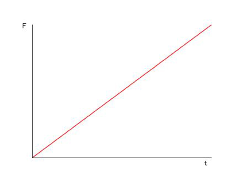
The load-controlled indentation mode is the most common type of indentation for simple and efficient hardness and elastic modulus measurement. It is described in detail in the ISO 14577 standard. A load-controlled indentation measurement consists in performing indentation measurement in which the loading and the unloading rates can be defined independently. Thanks to this mode, different loading types can be chosen, allowing the user to either accelerate the total test time or to analyze the response of different materials to different loading and unloading rates.
The linear loading is the most commonly used loading type. It can be used for most of the regular indentation testing applications.
The loading of the indenter follows the following formula:
$$F = k.t$$
Equation 10
In this formula k refers to the loading rate, usually expressed in [mN/s]. Supposing that the hardness is constant, the depth follows a square root evolution versus time ($F\sim{\sqrt{h}}$).
The recommended loading time given in ISO 14577 and ASTM 2808 is 30 seconds but when testing non-viscoelastic materials and for time-reducing purposes this value can be reduced.
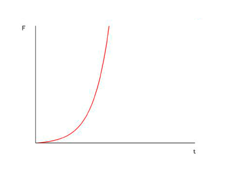
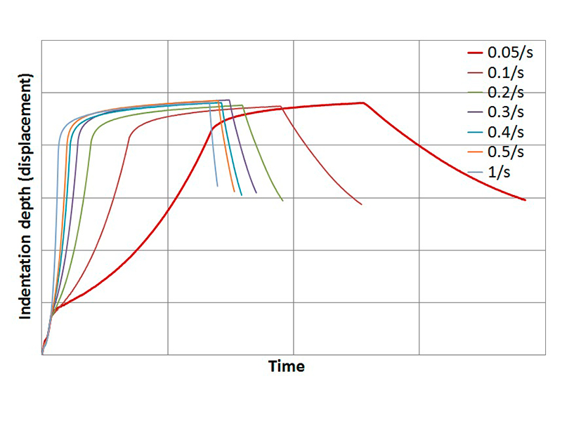
Constant strain rate loading
Viscoelastic materials, including polymers, exhibit mechanical properties dependent on strain rate, which expresses the material strain per unit of time. In order to compare samples of that material group, a constant strain rate must be kept during indentation measurements. This type of indentation control is based on the following equation:
$$\frac{dP}{dt} = const.$$
Equation 11
Using different constant strain rates can be advantageous for observing the creep response and also for finding optimal indentation conditions to reduce the effects of loading time on the elastic modulus in the case of viscoelastic materials.
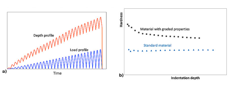
Cyclic loading indentation
Indentations with cyclically applied loading during one procedure can be particularly useful for obtaining depth profiles of hardness or elastic modulus on materials with graded mechanical properties such as functionally graded materials (FGM) or in multilayer coated systems. The mechanical properties of such materials are graded from the surface toward the load-bearing substrate or inner material. Cyclic indentation procedures allow characterization of the hardness and elastic modulus as a function of indentation depth. The loading/unloading in each cycle can be either defined as a function of load or depth.
Indentation in depth control modes
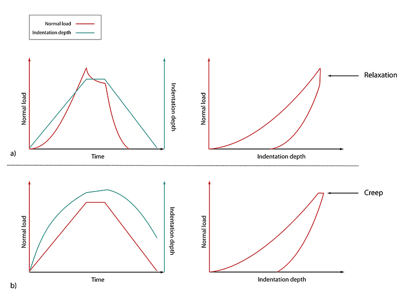
Some measurements might require indentation in “depth control” rather than in “load control” mode. A typical example is studying the pop-in effect for compressing micropillars. In these measurements the pillar suddenly deforms, which is much better visible in the drop of the compressing load as the load is temporarily decreased. The full depth control mode also allows the measurement of relaxation for materials with time-dependent properties such as polymers or hydrogels thanks to a constant depth at the maximum depth: as the material relaxes, the load on the indenter is decreasing. The “depth control” mode enables a specified maximum indentation depth to be reached by controlling the insertion speed and withdrawal speed (in m/min) of the indenter.
Figure 11 compares the different curves obtained with a “depth control” and a “load control” mode.
Figure 11a) shows an example of linear loading using a depth control. The indentation depth is servo-controlled all along the testing sequence and the resulting force evolution is measured. In this example, a hold of the maximum indentation depth was defined in order to measure the sample’s relaxation, in other words the evolution of the normal load over time that must be applied to maintain the defined indentation depth.
Figure 11b) presents a load-controlled linear loading. The normal load is servo-controlled and the resulting indentation depth evolution is monitored. Holding a force during a defined amount of time will allow characterization of the sample’s creep behavior, which is in practice the evolution of the indentation depth over time under the defined normal load.
Dynamic Mechanical Analysis
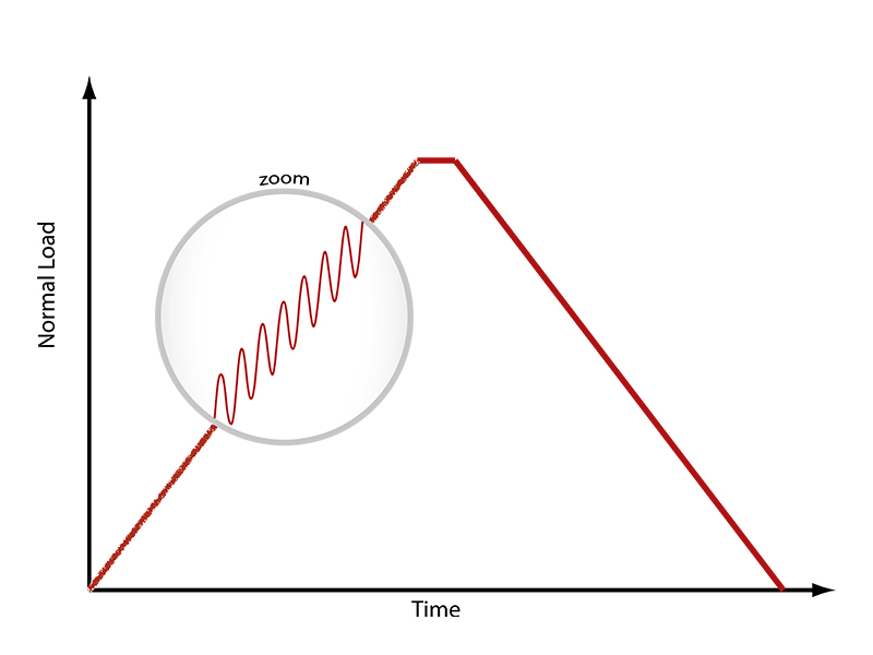
When analyzing the behavior of time-dependent materials such as polymers, indentation testing can provide great inputs thanks to the use of a dynamic mode. This technique, introduced by Oliver and Pharr, allows for a continuous measure of stiffness of the materials during the loading process by using a low-magnitude oscillating force superimposed onto the quasi-static force signal (Figure 12).
If oscillation amplitudes are small enough, it can be assumed that the sample deformation keeps within the linear viscoelastic regime during the “sinus” mode.
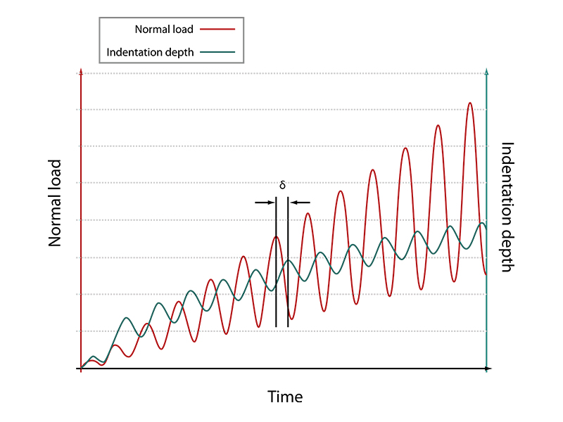
During a measurement, if a force oscillation is applied on the sample at a specific frequency, it will generate oscillations on the displacement signal with a phase angle δ (Figure 13).
The viscoelastic response of the tested material can be modeled using a spring having a stiffness S, which exhibits the elastic behavior, coupled in parallel with a dashpot having a damping factor D that models the viscous behavior of the sample.
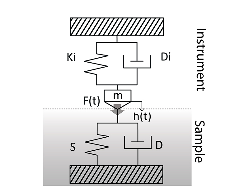
The dynamic mechanical model presented in Figure 14 is used to describe the viscoelastic behavior of the sample.
The dynamic stiffness Ki, damping Factor Di as well as the oscillating mass m of the instrument are known (can be calibrated). Therefore, by measuring the half force (F0) and displacement amplitude (h0), the angular frequency of oscillation ω as well as the phase angle δ between the force and displacement oscillations, it is possible to calculate the dynamic sample stiffness S, and the dynamic sample damping D.
$$S = {\frac{F_0}{h_0}}cos{\delta}+{m\omega}^2-K_i$$
Equation 12
$$D={\frac{1}{\omega}}{\frac{F_0}{h_0}}sin\delta - D_i$$
Equation 13
The viscoelastic parameters (storage and loss modulus and loss tangent) are then calculated using the following equations:
$${E'}= {\frac{\sqrt{\pi}}{2\beta}} {\frac{s}{\sqrt{A_p}}}(1-\nu^2)$$
Equation 14
$${E''}= {\frac{\sqrt{\pi}}{2\beta}} {\frac{D_\omega}{\sqrt{A_p}}}(1-\nu^2)$$
Equation 15
$$tan\delta=\frac{E''}{E'}$$
Equation 16
Conclusion
Instrumented indentation has been established as the reference characterization of thin films or bulk material mechanical properties. Progresses made in instrumentation allow the accurate determination of, among others, the elastic modulus and hardness of various materials, from soft materials to very hard. The different servo-control modes and adjustable measurement parameters also enable the analysis of material specifics. Dynamic indentation measurements notably offer the advantage of measuring hardness and modulus over the depth of a sample as well as viscoelastic properties.
Finally, the quick measurement cycle and the automated calculation can be a great advantage in the use of instrumented indentation as a quality control.
References
- Oliver, W. and Pharr, G. (1992). An improved technique for determining hardness and elastic modulus using load and displacement sensing indentation experiments. Journal of Materials Research, 7(06), pp. 1564–1583.
- Oliver, W. and Pharr, G. (2004). Measurement of hardness and elastic modulus by instrumented indentation: Advances in understanding and refinements to methodology. Journal of Materials Research, 19(1), pp. 3–20.
- Fischer-Cripps, A. (2011). Nanoindentation. New York, NY: Springer-Verlag New York Inc.
- Swiss Association for Standardization (SNV) (2014). Metallic Materials - Brinell hardness test - Part 1 (ISO 6506-1:2014).
- International Standards Office (2017). ISO 4545-1 Metallic materials - Knoop hardness test. Geneva: ISO.
- International Standards Office (2016). ISO 6808-1 Metallic materials — Rockwell hardness test —. Geneva: ISO.
- International Standards Office (2018). ISO 6507-1 Metallic materials -- Vickers hardness test. Geneva: ISO.
- International Standards Office (2015). ISO 14577-1 Metallic materials -- Instrumented indentation test for hardness and materials parameters. Geneva: ISO.
- ASTM International (2015). ASTM E2546 - 15 Standard Practice for Instrumented Indentation Testing. Conshohocken: ASTM.
- Herbert, E., Oliver, W. and Pharr, G. (2008). Nanoindentation and the dynamic characterization of viscoelastic solids. Journal of Physics D: Applied Physics, 41(7) 074021, pp. 1-9