Basics of Dynamic Mechanical Analysis (DMA)
Dynamic Mechanical Analysis (DMA) is a characterization method that can be used to study the behavior of materials under various conditions, such as temperature, frequency, time, etc. The test methodology of DMA, which aims mainly at the examination of solids, has its roots in rheology (see also “Basics of rheology”), a scientific discipline that studies the viscoelastic properties of different materials from liquids to solids. In this text, the fundamental principles, the basics of DMA, different measurement modes, and measuring systems will be discussed.
What is DMA?
In DMA measurements, the viscoelastic material behavior of solid-like samples is analyzed. To determine the time- and temperature-dependent deformation or flow characteristics, the specimen is set under a certain sinusoidal stress (or strain) and the material’s response is measured.
| Important terms and variables for DMA measurements: |
||
| Term | elongation | rotation/shear |
| Modulus | E | G |
| Complex modulus | E* | G* |
| Storage modulus | E’ | G’ |
| Loss modulus | E’’ | G’’ |
| Loss factor | tanδ | tanδ |
| Strain | ε | γ |
| Stress | σ | τ |
| Angular frequency | ω | ω |
| Time | t | t |
For better readability, the sizes and variables for tensile load are used in the article, unless otherwise necessary. |
||
What can DMA tell us?
In DMA measurements, the viscoelastic properties of a material are analyzed. The storage and loss moduli E’ and E’’ and the loss or damping factor tanδ are the main output values. Depending on the test setup, it is possible to make statements about several different material characteristics like physical properties (glass transition temperature Tg, molecular motions, crystallization, curing/crosslinking, etc.), mechanical properties (static and dynamic moduli, damping behavior, creep and relaxation behavior, etc.) as well as long-term material behavior (time temperature superposition (TTS)).
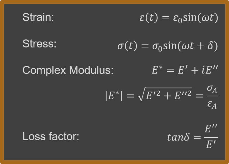
| Complex modulus |E*| – MPa Ratio of stress and strain amplitude σA and εA; describes the material’s stiffness Storage modulus E’ – MPa Measure for the stored energy during the load phase Loss modulus E’’ – MPa Measure for the (irreversibly) dissipated energy during the load phase due to internal friction. Loss factor tanδ – dimension less Ratio of E’’ and E’; value is a measure for the material’s damping behavior |
How does DMA work?
A specimen of the material to be examined is subjected to a certain sinusoidal stress or strain (axial or torsional deformation), and the reaction of the material is measured (Figure 1). An ideally elastic material reacts immediately, without any delay. The sinusoidal stress and strain curves show no phase shift, thus δ is zero. The stress and strain curves of an ideally viscous material show a phase shift angle of δ = 90 °. And as the term viscoelasticity suggests, the behavior of viscoelastic materials is a mixture of the two. Thus, the phase shift angle is 0° < δ < 90°.
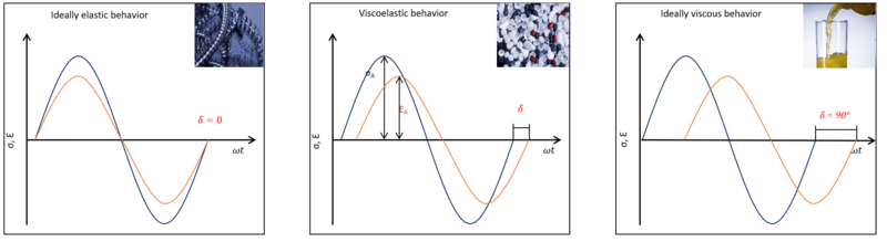
In Figure 2, important terms and their mathematical definitions are depicted.
Common DMA measurements
In addition to the variation of the mechanical stress amplitude and frequency, which is given by the linear or rotational drive of the DMA instrument, environmental parameters such as temperature or relative humidity can be set by means of an environmental test chamber.
Amplitude sweep (AS)
An amplitude sweep measurement is performed to determine a material’s linear viscoelastic (LVE) range. Here, mainly elastic (reversible) deformation occurs, which is highly relevant for all types of DMA analysis, as it enables the measurement of correct and absolute values without destroying the structure of the sample.
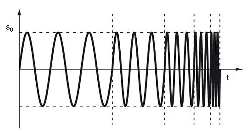
Amplitude sweep tests are performed at a constant temperature and frequency, whereas only the applied strain amplitude is varied within certain limits. Figure 3 illustrates a representative curve for an amplitude sweep. Storage and loss modulus as functions of deformation show constant values at low strains (plateau value) within the LVE range.
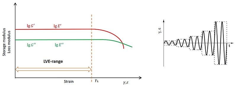
Right picture: Schematic profile of the applied deformation during the test
Frequency sweep (FS)
The frequency sweep generally provides information about time-dependent material behavior in the non-destructive deformation range. During the test, the frequency is varied, whereas the temperature and the applied strain or stress are kept constant. If necessary, a variation of the strain is possible within the LVE range. It is often combined with a temperature sweep to generate a master curve used for time temperature superposition (TTS).
Temperature ramp
DMA measurements with a temperature ramp are performed to determine transition temperatures (regions) of the specimen. For polymers, the glass transition temperature (Tg) is of particular interest. The different approaches to determine Tg will be discussed in the corresponding section.
Measurements including a temperature ramp are usually performed under a constant frequency (for example 1 Hz) and constant stress or strain. Within the LVE range, a variation of the applied strain is possible.
Humidity sweep
The surrounding relative humidity may have a major impact on mechanical properties of a sample too. These tests are usually performed at constant temperature and frequency. For some samples, a variation of the deformation makes sense in order to increase the accuracy of the measured curve. Nevertheless, it is important to stay within the LVE range.
Time sweep
In this kind of test, temperature and frequency are kept constant and the material behavior is investigated over time. E.g. it is used to investigate curing reactions of resins. In these tests, the material behavior can be analyzed from a liquid to a solid state. Since the material properties of liquid and solid samples behave very differently, a variation of the deformation (within the LVE range) can help to increase the accuracy of the measurement.
Thermal transitions
Using a DMA device, thermal transition temperatures can be determined with a test specification including a temperature ramp. These transition temperatures are of special interest for polymers because they show significant changes of their stiffness at certain temperatures. To make a suitable material selection for a certain application, it is of major importance to know the temperature-dependent material behavior of polymers.
The temperature-dependent behavior of a typical amorphous thermoplastic polymer is shown in Figure 5.
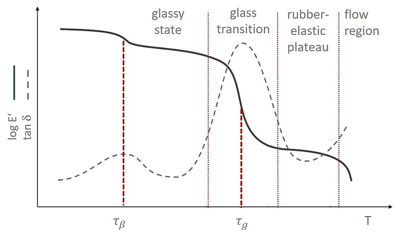
As shown in the diagram, transitions actually do not occur at one exact temperature, but within a certain temperature range where the material properties change. Therefore, there are different approaches to determine the glass transition temperature:
- Peak of the tanδ curve
- Peak of the E‘’ curve
- Step method on E’ curve
- Inflection point method on E´ curve
All these methods have their pros and cons and lead to slightly different results. So it’s important to use the same method when comparing different materials. It’s also essential to keep in mind that transition temperatures are transition areas and not sharply distinct values.
DMA operation modes
Since DMA systems can analyze a wide range of different materials, different measuring systems and different types of load are required.
Types of load
- Tension
- Bending
- Torsion/shear
- Compression
For DMA tests in tension, bending, and compression, classical stand-alone DMA systems equipped with a linear drive can be used. Here, the sample is loaded with an axial force. For measurements in torsion or shear, a rotational drive is needed.
Please note: Different types of load (axial force or rotational load) lead to different moduli. The Young’s Modulus or tensile modulus (also known as elastic modulus, E-Modulus for short) is measured using an axial force, and the shear modulus (G-Modulus) is measured in torsion and shear. Since DMA measurements are performed in oscillation, the measured values are complex moduli E* and G*. These two values are connected via the Poisson’s ratio ν: $G^* = {E^* \over 2(1+ν)}$ for isotropic materials.
This means that, if the Poisson’s ratio of the analyzed material is known, it is possible to convert results from one kind of test to the other. On the other hand, it is also possible to determine the Poisson’s ratio when G* and E* of a material can be measured.
Please note: Due to the different determination methods of E and E* (static vs. dynamic), the values for one and the same material are not identical. Usually, the values of the complex modulus are higher than the static values.
Measuring systems
As mentioned above, the range of materials that can be tested by using DMA systems is enormous: from very low modulus materials like very soft low weight polymer foams (~0.01 to 0.1 MPa) to elastomers and thermoplastics (~0.1 to 50,000 MPa) and fiber-reinforced polymers (~10,000 to 300,000 MPa). To analyze these very distinct types of materials, different measuring systems are needed:
Table 1: Overview of DMA measuring systems, the according deformation modes, and examples for suitable samples
| PP (parallel plates) | Foams | ||||
| SRF (solid rectangular fixture) | Thermoplastics | ||||
| SCF (solid circular fixture) | Thermoplastics | ||||
| UXF (universal extensional fixture) | Polymer films | ||||
| TPB (tree point bending) | Ceramics | ||||
| CTL (cantilever bending) | Elastomers |
Material selection based on the characteristics deduced from dynamic mechanical analysis
Figure 6 provides an overview of the loss modulus tanδ and the Young’s modulus. They were deduced via dynamic mechanical analysis of different materials and material classes at a temperature of 30 °C.

Table 2: Abbreviations of terms found in the chart
| Abbreviation | Complete term |
| IR | Isoprene |
| VLD | Very low density |
| elPu | Polyurethane elastomers |
| MD | Medium density |
| LD | Low density |
| EVA | Ethylene-vinyl acetate |
| HD | High density |
| PTFE | Polytetrafluoroethylene (Teflon) |
| PE | Polyethylene |
| PP | Polypropylene |
| ABS | Acrylonitrile butadiene styrene |
| PMMA | Poly(methyl methacrylate) |
| GFRP | Glass fiber reinforced polymers |
| CFRP | Carbon fiber reinforced polymers |
| Mg | Magnesium |
| Ti | Titanium |
| WC | Tungsten carbide |
| SiC | Silicon carbide |
| Si3N4 | Silicon nitride |
| Cu | Copper |
| Al | Aluminum |
The effort to meet the multitude of technical requirements related to all conceivable products or components is accompanied by an almost unmanageable number of materials to choose from. These materials stem from different material classes like metals, ceramic materials, plastics, etc. Illustrations like the one above enable selection of suitable material classes and materials for specific applications. This can help identify possible alternatives not initially considered.
The diagram shows, e.g. that technical ceramics achieve very high modulus values, but have hardly any damping capacity. For applications requiring a combination of high deformation resistance and moderate damping capacity, metallic materials or polymer composites are better suited, as shown in the diagram. If, in contrast, good damping behavior is of major importance in an application, but the mechanical load-bearing capacity is negligible, materials from the field of polymer foams are the right choice.
This way, a product designer can see at a glance which material class meets the mechanical requirements of a specific application, to perform a pre-selection of appropriate materials. For a material scientist who wants to examine a material more closely, the diagram permits an estimation of the expected mechanical properties. This can be of great value when selecting suitable measuring systems and creating test specifications.