How to measure viscosity
The principles introduced in this section represent a cross-section from traditional to technically advanced methods.
Gravimetric capillaries and flow cups
True to their name, gravimetric capillaries – as well as flow cups – rely on gravitational force as the drive. The resulting quantity is kinematic viscosity. Flow or efflux cups and gravimetric capillaries should only be used for measuring the viscosity of ideally viscous liquids.[1]
How the gravimetric flow principle works
Take a capillary with precisely specified dimensions (inner diameter, length) and an equally precise distance given by two marks. Let a known quantity of liquid flow through this capillary and measure the time the liquid level takes to travel from one mark to the other. The measured time is an indicator for viscosity (due to the velocity of flow depending on this quantity). To obtain kinematic viscosity (v = ny), multiply the measured flow time (tf) by the so-called capillary constant (KC). This constant needs to be determined for each capillary by calibrating the capillary, i.e. by measuring a reference liquid of known viscosity.
$$v = K _{C} {\cdot} t _{f}$$
Equation 1: Flow time of sample multiplied by the gravimetric capillary constant gives kinematic viscosity.
The flow time must not fall below a specified minimum, otherwise the flow inside the capillary will no longer be laminar.
If a flow cup is used, the principle works as described above, but instead of exact capillary dimensions, the volume of the cup and its outlet capillary need to be accurately defined. As a rule, the equations for getting viscosity from the flow time are empirically determined for each cup by way of calibration tests with viscosity reference standards.
Its simplicity is the main strength of this principle and also the reason why it appears in many standards and standardized practices. Gravity as drive is present everywhere on earth, free of charge. It does not require additional technical equipment or maintenance.
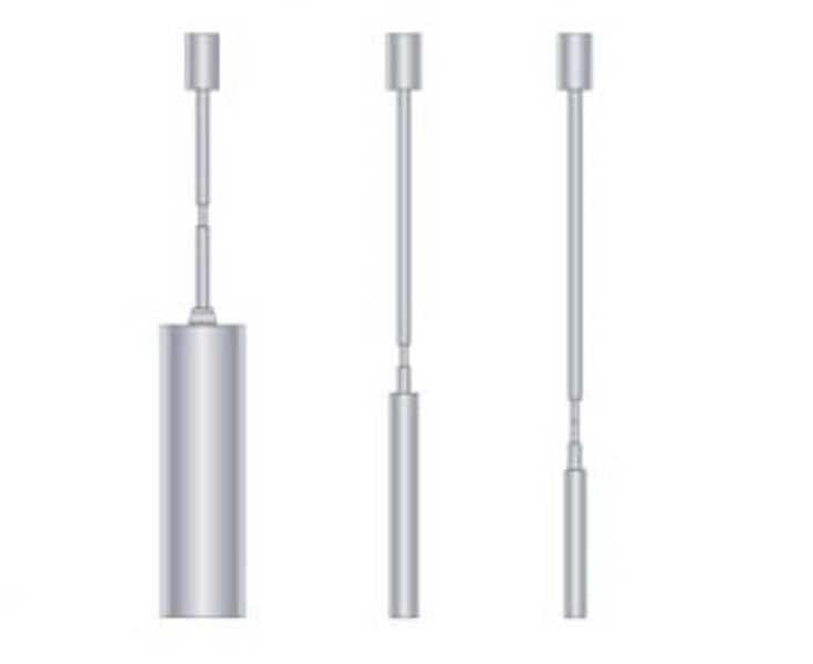
On the other hand, you cannot alter gravity as the driving force. One disadvantage is that it is not strong enough to test high-viscosity substances. Another drawback is that you need several capillaries to cover a wide viscosity range: Due to the one constant driving force, you have to vary the dimensions of the capillaries. For example, each Ubbelohde capillary serves for a range defined by its minimum viscosity times factor 5 (e.g. 0B: 1 mm²/s to 5 mm²/s). Sixteen capillaries cover a total measuring range from 0.3 mm²/s to 100 000 mm²/s. Figure 2 shows an Ubbelohde capillary.

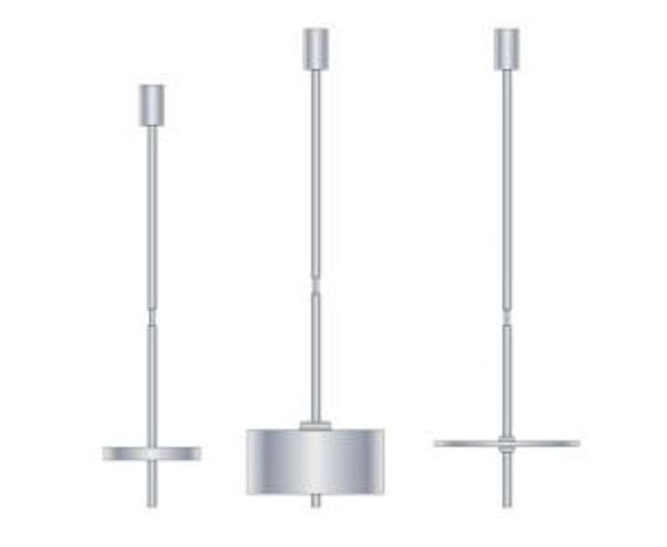
Types of available glass capillaries
Generally, gravimetric capillaries are made of glass. They are divided into direct-flow or reverse-flow models.
Direct-flow capillaries feature the sample reservoir below the distance marks, while in reverse-flow types the reservoir is placed above. This construction enables users to measure even opaque fluids. Some reverse-flow tubes are equipped with three measuring marks. Consequently, you get two flow times, which also gives you determinability.
Typical representatives of glass capillaries

Figure 2: Established types of glass capillaries:
- Ostwald capillary (named after Wilhelm Ostwald, 1853 – 1932, German chemist[2])
- Ubbelohde capillary (named after Leo Ubbelohde, 1877 – 1964, German chemist[3])
- Cannon-Fenske capillary (a modified Ostwald capillary, designed by Dr. Michael R. Cannon, American scientist, inventor, and educator, and Merrell Robert Fenske, 1904 – 1971[4]
- Houillon capillary (Standard ASTM D7279 describes measurement using this capillary type)
Manual gravimetric capillaries
With traditional glass capillary viscometers, the flow time is taken manually utilizing a stop watch, which demands full concentration and exact work from the operator. In addition, reliable thermostat baths as well as suitable bath liquids are required.
Automatic gravimetric capillary viscometer
To save working time and material resources, automatic varieties of gravimetric capillary viscometers were developed. The most advanced models automatically fill, measure, clean, and dry. Furthermore, automatic performance excludes human mistakes, such as reading errors. The greater part of automated capillary viscometers features special capillaries working with less measuring volume than the original types, or covering an extended viscosity range. These capillaries are not in accordance with the original standards, but offer comparable precision.
Such automatic viscometers mainly employ liquid baths, sometimes combined with a thermoelectric system, for temperature control.
Types of flow cups
Flow cups are used for testing all kinds of coatings, but also ceramic suspensions, drilling fluids, and even hot bitumen. Depending on the specific application, a different flow cup is utilized.[5]

Figure 3: Some types of flow cups.[5]
- ISO 2431
- DIN 53211
- Ford
- Zahn
- Engler
- Shell
Pressurized capillary viscometers
Apart from capillary viscometers driven by gravity, there are also pressurized devices in use. We distinguish between three ways of applying pressure: by using a weight, a motor, or gas pressure.[6]
Capillary viscometers utilizing a weight
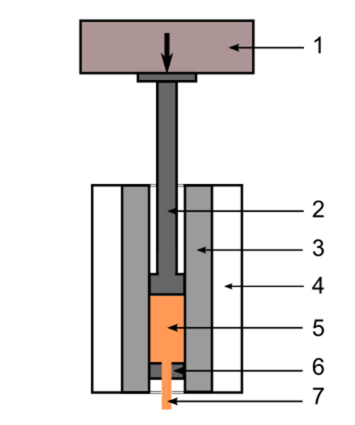
<li>Steel piston</li>
<li>Steel cylinder</li>
<li>Heating and insulation</li>
<li>Polymer melt</li>
<li>Die</li>
<li>Extrudate</li></ol>
This type of instrument plays a major role in checking polymer melts. The device returns the MFR (melt mass flow rate) in [g/10 minutes] or the MVR (melt volume flow rate) in [cm³/10 minutes]. These parameters help to assess the quality of the melt and to predict its behavior when processing it. Consequently, such an instrument is also named MFR or MVR tester.[6]
How pressurizing by weight works
A defined weight on top of a piston is pulled down by gravity. The steel piston glides down inside a vertical steel cylinder, which contains the sample. The sample then has to pass through an extrusion die (i.e. capillary) at the bottom of the cylinder. ISO 1133 states the dimensions of cylinder, piston, and die as well as the approved weight pieces. In such devices, the polymer sample is exposed to medium shear stresses (from 3 kPa to 200 kPa) and medium shear rates (from 2 s-1 to 200 s-1).[6]
High-pressure capillary viscometers with electric drive
Such a viscometer works in the same way as a weight-driven instrument (see the above section). However, the weight is replaced by a driving motor, which realizes high shear stress values (up to 900 kPa) and medium to high shear rates (around 1,500 s-1). Typical applications are highly viscous substances, such as polymer melts, and also PVC plastisols, greases, sealants, adhesives, and ceramic masses.[6]
Capillary viscometers utilizing gas pressure
These devices feature a glass or steel capillary of exact inner diameter and length. The inner diameter lies between 0.2 mm and 1 mm, while the length ranges from 30 mm to 90 mm. Gas forces the sample through the capillary at a preset pressure. This method can operate in a shear rate range up to 1,000,000 s-1. Shear stress values, however, do not exceed the medium range (a typical value would be 25 kPa). The dimensions of the capillary show that this kind of apparatus is designed for medium- to low-viscosity substances: mineral oils, paper coatings, and dispersions, and for polymer solutions used to produce synthetic fibers on spinning machines.[6]
The sample under test can be in direct contact with the driving gas, or via a flexible membrane. For example, pressurized air or an inert gas such as technical nitrogen is employed.[6]
Falling-ball and Rolling-ball viscometers
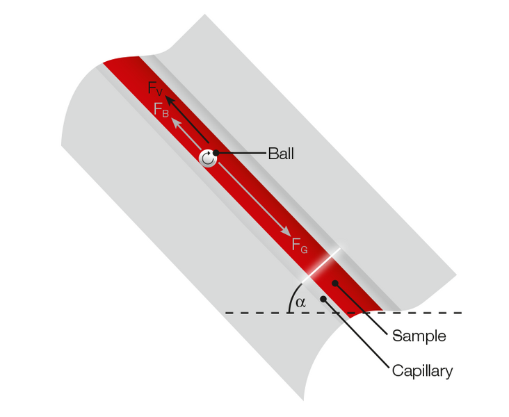
A falling-ball / rolling-ball viscometer does not measure a liquid’s flow time, but the rolling or falling time of a ball. Gravity acts as the driving force.
How the rolling-ball principle works
A ball of known dimensions rolls or falls through a closed capillary, which contains the sample liquid. A preset angle determines the inclination of the capillary. The time it takes the ball to descend a defined distance within the fluid is directly related to the fluid’s viscosity.
The inclination angle of the capillary allows for adjusting the driving force. A too steep angle results in a too high speed of the ball, which leads to turbulent flow conditions and faulty results.
Other forces than the ones named above are negligible, provided there is laminar flow. A portion of the gravitational force, which depends on the angle, drives the ball downwards. As opposing forces, the buoyancy inside the sample and the viscous forces of the liquid slow the ball down. It follows that for identical inclination angles the rolling time increases with the viscosity of the sample.
These three principal forces determine the viscosity equation:
$$\eta = K \cdot (\rho_b - \rho_s) \cdot t_r$$
Equation 2: Rolling time of the ball multiplied by the density difference of ball and sample and the adjustment constant K gives dynamic viscosity.
η ... dynamic viscosity [mPa, s]
K ... proportionality constant [1]
ρb ... ball density [g/cm3]
ρs ... sample density [g/cm3]
tr ... ball rolling time [s]
$$F_G = m \cdot g = \rho \cdot V \cdot g$$
Equation 3: Density and dimensions of the ball influence the gravitational force acting on the ball.
m ... mass [kg]
g ... acceleration of gravity [m/s2]
ρ ... density [kg/m3]
The ball’s density plays a vital role, as it is included in the equation for the gravitational force (see Equation 3). By replacing the density of the liquid with the ball’s density in Equation 3, you obtain the buoyancy. Consequently, both density values (ρb, ρs) are required to calculate the viscosity. The proportionality constant (K) results from an adjustment with a viscosity reference standard.
Types of falling-ball and rolling-ball viscometers
Devices operating at inclination angles between 10° and 80° are usually defined as rolling-ball viscometers. If the inclination angle exceeds 80°, the instrument in question is a falling-ball viscometer. An exception to this rule is the Hoeppler viscometer, a falling-ball instrument which states an inclination angle of exactly 80°.
The Hoeppler principle (Fritz Höppler, 1897 – 1955, German chemist, who designed this falling-ball viscometer in 1933[7]) conforms to DIN 53015 and ISO 12058. Temperature control is realized via liquid bath thermostat, while an operator manually performs measurement and cleaning.
Certain devices use other falling objects than balls, for example rods or needles. The original principle has also been varied: The so-called bubble viscometer measures the time it takes an air bubble in the fluid to rise. The oscillating piston viscometer of ASTM D7483 replaces gravity as the driving force by electromagnetic force, which draws a magnetic cylinder through the fluid.
Rolling-ball microviscometer
The rolling-ball microviscometer implements a further development of the Hoeppler principle. This device replaces the falling tube by considerably smaller micro capillaries, reducing the required amount of sample volume. Depending on the sample’s viscosity, the filling quantity can be as low as 100 µL. Micro capillaries are available made of glass or of PCTFE, which even allows for testing fluids which corrode glass. Inductive sensors register the rolling time, while thermoelectric temperature control and adjustable inclination angles enhance the instrument’s flexibility.
Generally, a microviscometer is best suited for measuring liquids in the low-viscosity range.
Rotational viscometers
Rotational viscometers push the upper limit of the potential measuring range further than gravity-based devices. They use a motor drive, which is significantly stronger than the earth’s gravitational force. Therefore, they are suited for measuring more highly viscous substances. The resulting quantity is dynamic viscosity, sometimes also referred to as shear viscosity.
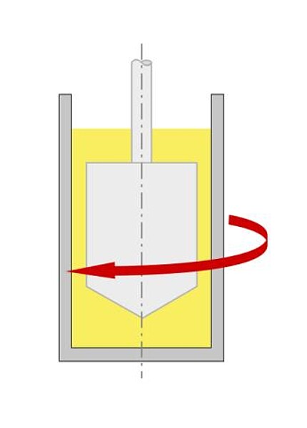
Basically, a typical rotational viscometer is a cup containing the sample; the cup is matched with a so-called measuring bob that is placed in the substance under test. Depending on which part is driven, there are two principles:
- the Couette principle
- the Searle principle
How the rotational principles work (Searle and Couette)
Searle principle
The motor drives the bob inside the fixed cup. The rotational speed of the bob is preset and produces a certain motor torque that is needed to rotate the measuring bob. This torque has to overcome the viscous forces of the tested substance and is therefore a measure for its viscosity. When testing low-viscosity liquids, excessive rotational speed could cause turbulent flow due to centrifugal forces and inertia.
Most commercial rotational viscometers incorporate this principle, which is named after G.F.C. Searle (George Frederick Charles Searle, 1864 – 1954, a British physicist and teacher, who designed a rotational viscometer with rotating concentric inner cylinder in 1912[8]).

Couette principle
The motor drives the cup while the bob is stationary. Such a system minimizes the risk of turbulent flow. The crucial point in this setup is how to implement the cup drive: the driving shaft needs to be leak-tight against liquid used for temperature control (if any). Due to that difficulty, there are only few classic Couette instruments on the market.
M. M. A. Couette lent his name to this principle (Maurice Marie Alfred Couette, 1858 – 1943, French physicist, who developed the “drag-flow” viscometer in 1888[9]).
Physics of the Searle principle
The motor turns a measuring bob or spindle in a container filled with sample fluid. While the driving speed is preset, the torque required for turning the measuring bob against the fluid’s viscous forces is measured.

Figure 8: Rotational viscometer - Searle principle
- … Motor and measuring unit
- … User interface
- … Stand
- … Spindle/bob axis
- … Sample-filled cup
- … Measuring spindle/bob (rotor)
Types of rotational viscometers
Besides the two varieties of the rotational measuring principle, there are manifold designs of measuring bobs. This diversity arises from a great number of different applications within a viscosity range from 1 mPa.s up to 4 000 000 mPa.s. Some systems are even suitable for testing inhomogeneous samples such as crunchy peanut butter, yogurt containing pieces of fruit, or building materials.
Find examples of some typical measuring bobs in the paragraph “Measuring Bobs for Rotational Viscometers”
We can further distinguish between types of rotational instruments by the way the torque is measured:
- Spring instruments
- Servo motor instrument
Spring instruments
Spring instruments feature a two-part axis connected via a spiral spring and a pivot. The motor – usually a stepper motor – turns the upper part of the central axis. One end of the spring is fixed to it. The spring’s other end connects to the bob side of the axis. The pivot stabilizes the construction. One part of the pivot is also fixed to the motor axis, while its counterpart connects to the bob. In order to minimize friction, the counterpart only rests on one point. The rotation of the bob deflects the spring in proportion to the torque representing the sample’s viscosity. Two optical sensors detect the deflection utilizing slotted discs. In figure 8, the parts connected to the motor are marked light blue, the parts on the bob side light brown.
In case of low viscosity substances, the spring needs to be sufficiently sensitive, while for samples in the high-viscosity range a more robust spring is required. Consequently, one and the same apparatus cannot serve a wide measuring range. However, such a spring system is highly sensitive to low torque values.

Figure 9: Spring viscometer: A spiral spring connected to both the motor and the rotating bob registers the motor torque as a measure of viscosity.
1 … Motor
2 … Slotted disc on motor side
3 … Position sensor on motor side
4 … Spiral spring
5 … Pivot
6 … Position sensor on bob side
7 … Slotted disc on bob side
8 … Rotating measuring bob
Servo motor instruments
This instrument type is equipped with a servo motor and a high-resolution digital encoder. The motor turns the main shaft to which the measuring bob is attached. The encoder records the rotational speed. The resulting motor torque is related to the viscous forces of the tested sample. As the motor current is proportional to the torque, the viscosity is calculated using motor current and rotational speed.
Such a device is not limited by the properties of a mechanical spring. Encoder and motor both support wider speed and torque ranges and, consequently, a wider viscosity range than a spring viscometer. The stiff axis makes the system more resistant to damage than the pivot-based system. On the other hand, the friction of the motor and its bearing reduces measurement accuracy, especially in the low-viscosity segment and at low speeds.
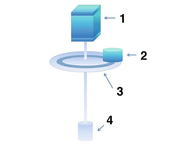
Figure 10: Servo motor viscometer: The motor current is proportional to the motor torque, which represents the viscosity of the sample.
1 … Servo motor providing highly precise measurement of the motor current
2 … High-resolution optical encoder counting the rotational speed
3 … Encoder disc
4 … Rotating measuring bob
Measuring bobs for rotational viscometers
An extensive quantity of different measuring bobs serves to test various types of substances. Generally, the relation between bob size and sample viscosity is inversely proportional: The lower the viscosity is, the more voluminous the bob should be. However, most of these bobs come without defined geometry, which gives relative viscosity value[10] and reduces comparability of measurement results. Nor is it then possible to calculate shear rate and shear stress.
Coaxial cylinder systems
Coaxial (or concentric) cylinder systems are absolute measuring systems, which also conform to DIN and ISO. Mainly special adapters for rotational viscometers house such systems. Usually these adapters are intended for a small quantity of sample and additionally offer some kind of temperature control. Due to precisely defined geometries of the bob and its cup, they permit the operator to compute shear rate as well as shear stress and, consequently, absolute viscosity values[10].
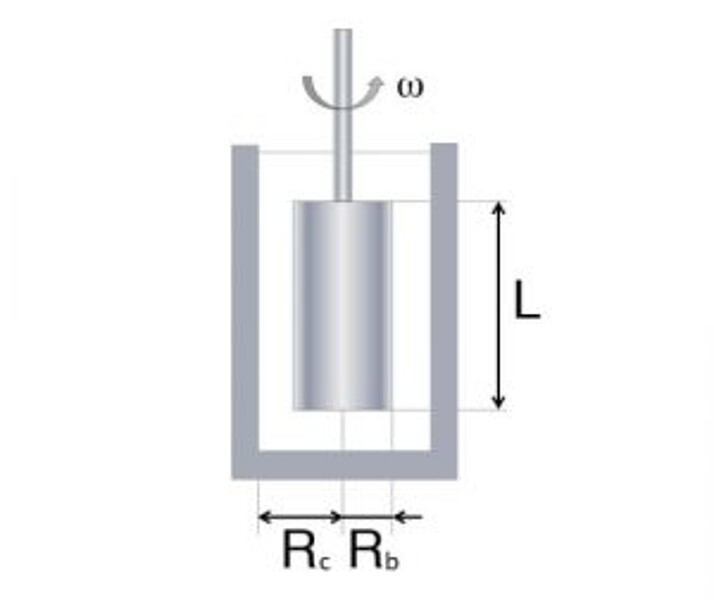
Figure 14: Coaxial cylinder geometry used with rotational viscometers. Precisely defined dimensions allow for calculating shear rate, shear stress, and absolute dynamic viscosity.
Rc ... radius of container [m]
Rb ... radius of bob [m]
L ... length of bob [m]
γ˙ ... shear rate [s-1]
ω ... angular velocity [rad/s]
τ ... shear stress [N/m2]
M ... measured torque [Nm]
η ... dynamic viscosity [Pa, s]
$$\dot{\gamma} = {2 \cdot \omega \cdot R_C² \over (R_C² - R_b²)}$$
Equation 4: Shear rate in coaxial cylinder systems.
$$\tau = {M \over 2 \cdot \pi \cdot R_b² \cdot L}$$
Equation 5: Shear stress in coaxial cylinder systems.
The equation for the shear rate on the bob’s surface contains the dimensions of the parts and the rotational speed (also named angular velocity). Shear stress depends on the measured torque, the bob’s radius and length. According to Newton’s Law[13], these parameters determine the dynamic viscosity.
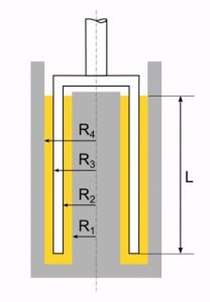
Double-gap cylinder systems
Double-gap systems[14] are a special form of concentric cylinders, specially devised for measuring low-viscosity liquids.
The cup is not a hollow cylinder, nor is the measuring bob a solid body. A second cylinder is placed in the center of the cup and the bob is shaped like an inverse cup that turns in the ring-shaped gap between the cup’s outer and inner walls. This construction maximizes the available bob surface in contact with the sample liquid, which means that you get a much larger shear area than in standard cylinder systems. Therefore, this system is able to detect low torque values as generated by low-viscosity samples.
DIN 54453 (withdrawn) states the following for the system’s dimensions:
R4/R3 = R2/R1 <= 1.15 … relations of radii
L >= 3 • R3; L … immersed length of the bob
Cone-plate and parallel-plate measuring systems
Cone-plate and parallel-plate systems[15] shear the sample under test in a defined gap between the fixed plate and the rotating bob. The bob is shaped as a cone or as a plate. Such systems adhere to standards (e.g. ISO 3219|1993 for cone-plate and ISO 6721-10|1999 for parallel-plate), which precisely establish approved geometries. For cones, an angle of 1° is recommended, but angles < 4° are permissible. The cone radius should be between 10 mm and 100 mm. For parallel plates, the standard demands that H << R. So, depending on the plate radius and the sample under test, H can range from 0.5 mm to 3 mm. Due to the narrow gaps, only a small amount of sample is required. However, a gap is open to the side so it follows that low-viscosity liquids may simply flow away, especially at higher rotational speeds, when turbulent flow and centrifugal forces occur.
The wedge-shaped gap caused by the cone results in the sample being submitted to constant shear rate over the entire gap – a significant advantage allowing for the measurement of absolute viscosity values.
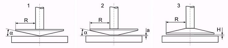
A truncated cone means that the tip of the cone looks as if it has been cut off. Of course, the geometry still adheres to strict specifications. Gap a between cone and plate is usually in a range between 50 µm to 210 µm. The absence of a cone tip avoids abrasion between cone tip and plate and eliminates friction between cone and plate. Both could influence measuring results unfavorably: the former, by changing the system’s geometry over time, the latter by falsifying torque values. An additional advantage is that with a truncated system even materials with particles can be analyzed, provided the particles are no larger than one fifth of the gap between cone and plate.
Cone-plate and parallel-plate systems are also suited for extensive rheological (oscillatory) tests.
SVM Viscometer
First introduced in 2001, the SVM Viscometer is a comparatively young device. It combines a wide measuring range with maximum precision. Standard ASTM D7042 establishes that this viscometer determines kinematic viscosity with accuracy equal to traditional gravimetric capillaries.
How the SVM Viscometer Works
The SVM Viscometer incorporates a modified Couette principle. Instead of a rotating cup, it employs a small-size tube containing the sample, whereas the original bob is replaced by a hollow, freely floating rotor. The entire system is located in a temperature-controlled copper block, which ensures stable conditions. A motor turns the tube at constant speed. As the sample moves with the encircling tube, the viscous forces of the sample drive the floating rotor. A combination of hydrodynamic lubrication[16] and centrifugal forces pushes the rotor to the center of the sample. The rotor holds a small permanent magnet that generates a rotating magnetic field. Any alternating magnetic field in an electrically conductive material such as copper induces eddy currents opposing their origin. This effect slows the rotor down, while the sample forces accelerate it. Once the rotor attains an equilibrium speed, this speed is an indicator for dynamic viscosity. An adjustment with viscosity reference standards relates the instrument’s internal data to correct viscosity values.
The magnet inside the rotor further serves to measure the rotor speed: A Hall-effect sensor counts the frequency of the rotating magnetic field.
The non-contact sensor technology along with the rotor that is free from friction are the basis for the flexible measuring range from 0.2 mPa.s to 30,000 mPa.s and the extremely precise torque resolution of 50 pNm.
Many applications, e.g. in the petrochemical industry, traditionally operate with kinematic viscosity. Therefore, a highly precise density measuring cell consisting of a metal U-tube oscillator[17] is also part of the SVM Viscometer. From simultaneously measured density and dynamic viscosity, the instrument calculates kinematic viscosity.
Advanced Information
The lower a liquid’s viscosity, the slower the rotor turns and the higher the speed difference between tube and rotor: Low-viscosity forces transfer only a small part of the preset tube speed to the rotor. Mathematically put, dynamic viscosity is inversely proportional to the speed difference between tube (n2) and rotor (n1).
$$\eta \sim {1 \over n_2 - n_1}$$
Equation 6: Dynamic viscosity is inversely proportional to the speed difference between tube and rotor.
For speed equilibrium, the driving torque of the rotor must equal its retarding torque.
$$M_D = M_R$$
$$M_D = K_1 \cdot \eta \cdot (n_2 - n_1)$$
$$M_R = K_2 \cdot n_1$$
$$\eta = {K \over {n_2 \over n_1} - 1} = {K \over {n_2 - n_1 \over n_1}} \rightarrow K = {K_2 \over K_1}$$
MD … driving torque of the rotor
MR … retarding torque of the rotor
n1 … rotor speed
n2 … tube speed
K1, K2, K … constants; K is determined during adjustment
Equations 7 to 10: Equilibrium between driving torque (related to viscosity) and retarding torque (electromagnetic forces).