Laser diffraction for particle sizing
Laser diffraction is one of the most common techniques for particle size analysis. It is based on the observation that the angle of (laser) light diffracted by a particle corresponds to the size of the particle. In a complex sample containing particles of different sizes, light diffraction results in a specific diffraction pattern. By analyzing such a pattern the exact size composition (i.e. particle size distribution) of the sample can be deduced.
Introduction
Diffraction (from Latin diffringere, 'to break into pieces') is a phenomenon of waves bending when encountering obstacles or slits. Any type of a wave – mechanical, such as sound and water waves, but also electromagnetic, such as light waves – can be diffracted.
Light diffraction has an analytical application to determine the size of the obstacle the light wave is running into. This analytical method is based on the fact that the angle of light diffraction is inversely proportional to the size of the obstacle (Figure 1). In practice, the light source used for such analysis is usually a laser, so the technique is commonly referred to as laser diffraction. In order for laser diffraction to work, the obstacles need to be small enough to be comparable to the wavelength of the laser. Such tiny obstacles are generally referred to as particles. Any small and distinct subdivision of matter can be a particle, e.g. a grain of a powder or a droplet in an emulsion.
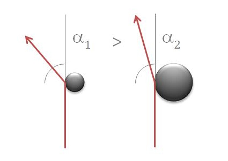
Figure 1: Schematic depiction of laser diffraction when the laser encounters obstacles small enough to be comparable to its wavelength. The diffraction angle of small particles (α1) is bigger than the diffraction angle of bigger particles (α2). Therefore, the complex diffraction pattern coming from different particle sizes in a sample is used to determine the particle size distribution (PSD).
Particle size determination
Diffraction
A laser diffraction experiment for particle size determination has a simple setup: The dispersed particles are first directed towards a laser beam (Figure 2). The beam gets diffracted by the particles at different angles depending on the particle size (Figure 1). The different angles of diffraction are seen as specific diffraction patterns (i.e. Airy pattern, Figure 3), which also depend on the particle size (Figure 4). The diffraction pattern is then detected and analyzed by a complex algorithm that compares the measured values to expected theoretical values (see chapter Detection and analysis). The result is a particle size distribution (PSD).
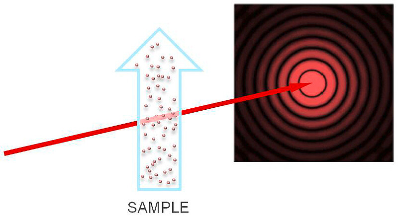
Figure 2: Illustration of laser diffraction in a particle size analyzer. The red arrow represents the laser beam, which shines through the sample (blue arrow).The concentric circles represent a simplified diffraction pattern.
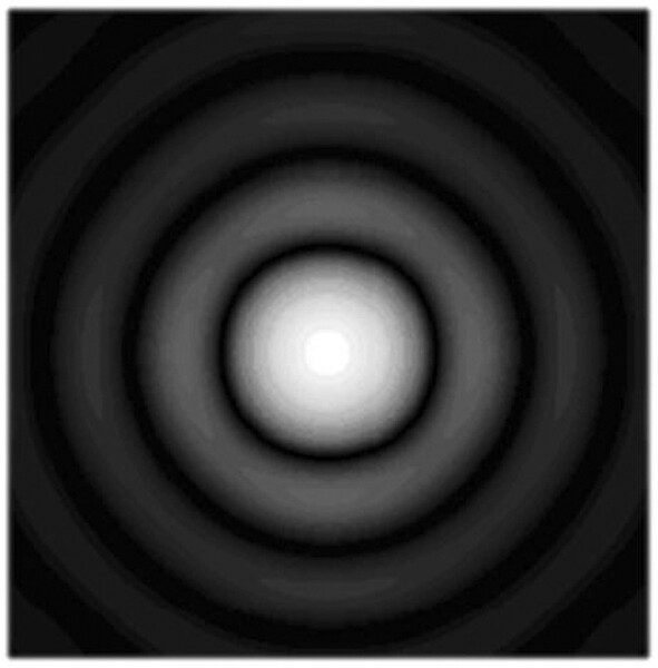
Figure 3: The visual result of light diffraction: The innermost circle is called the Airy disk. Together with the outer concentric rings it forms the so-called Airy pattern (or diffraction pattern).
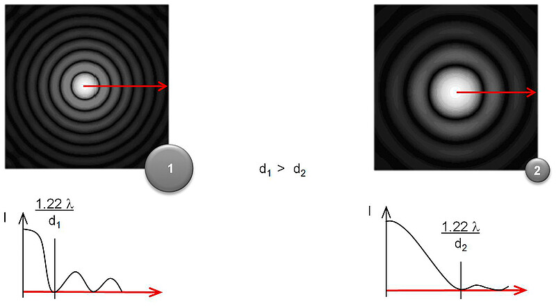
Figure 4: Simulation of diffraction patterns for two spherical particles. Particle a is twice the size of particle b. Above is a plot of the radial intensity of diffracted light through a cross-section (shown as a red arrow). As shown in the equations, the size of the Airy disk is directly proportional to the wavelength (λ), but inversely proportional to the size of the particle (d). That means that bigger particles exhibit smaller Airy disks, i.e. more “dense” diffraction patterns.
Dispersion
In order to get a clear diffraction, it is necessary to have a proper dispersion of the sample. This means that each particle should be visible as a single particle in front of the laser, moving through either liquid medium or air. Usually a sample should be analyzed in a state relevant to its application, i.e. it should be measured in liquid mode if the final product is a liquid dispersion and in dry mode if the final product is a powder.
In liquid mode the particles are dispersed in a liquid and pumped into a glass measurement cell which is placed in front of the laser. The sample keeps circulating until the measurement is done. The liquid dispersion unit is usually equipped with a mechanical stirrer with adjustable speed and with a sonicator with adjustable duration and power.
In dry mode the powder is put into motion either by compressed air or by gravity, creating a dry flow which is positioned in front of the laser beam. The sample de-agglomerates (breaks down into smaller sized particles) as particles collide with each other or with the wall of the dispersion unit.
Detection and analysis
The diffraction patterns shown so far represent the ideal case of a single-sized population of perfectly spherical particles (Figure 2, Figure 3, Figure 4). However, real samples consist of a number of particles of different sizes and often also different shapes. As an outcome, each particle shows a specific diffraction pattern, and they all overlap resulting in an uneven patch of light rather than a distinguishable pattern (Figure 5). This chapter will explain how laser diffraction particle size analyzers convert the detected intensities into information about particle sizes contained in the sample.

Figure 5: Intensity plot: Overlapping diffraction patterns of a sample containing particles of different sizes (left), and a sum of diffraction patterns, i.e. intensities actually measured by the detector (right).
Raw data acquisition
In Figure 6 the actual detector of a particle size analyzer is shown. Its shape enables it to detect a wedge of the circular diffraction pattern (Figure 3). Each photosensitive area will receive a different intensity of light, depending on the specific diffraction pattern. To detect angles too big for the wedge detector, additional individual detectors are usually placed.
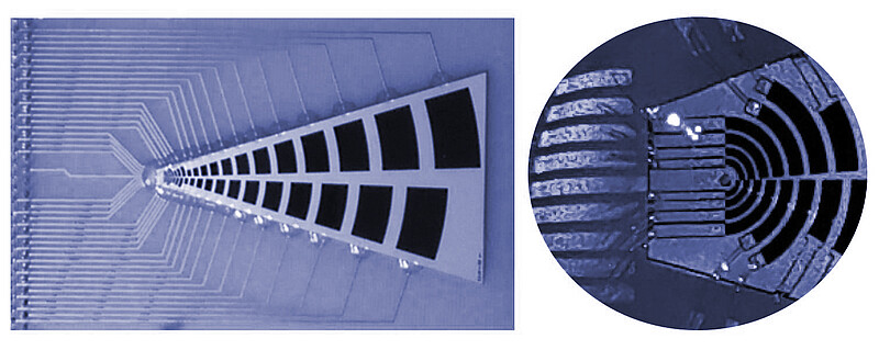
Figure 6: An example of a main detector of a laser diffraction instrument. At the center of the wedge there is a tiny hole allowing the undiffracted laser beam to pass through (close up photo on the right). The black blocks are the photosensitive areas which detect the intensity of diffracted light at different angles.
Data analysis
Once the instrument has recorded an intensity plot (Figure 5), the next step is to distinguish the individual diffraction patterns it consists of. The matrix illustrating the general principle is shown in Figure 7. The algorithm estimates proportions of the size classes in the total volume, i.e. particle size distribution (PSD) by comparing the measured data to the expected theoretical values for different size classes.
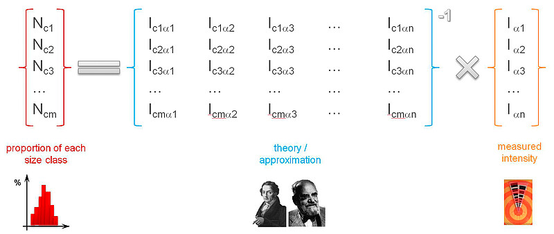
Figure 7: Matrix representing the principle of extracting particle size distribution (PSD) from raw intensity data. Raw intensity (I) data is shown in orange brackets and divided into portions measured by each detector, i.e. at each angle from α1 to αn. The blue part of the equation represents the theoretical part, i.e. the expected intensities for each size class (c1 to cm) and at each angle of detection (α1 to αn). By comparing the theoretical with actual intensities, PSD can be calculated. This result is shown in red brackets, where N stands for the relative proportion of each size class (c1 to cm) in the total volume.
The theoretically expected values for different particle sizes are illustrated as a 3D graph in Figure 8. The graph shows that for very small particles in the nano-range there is practically no diffraction pattern visible. For such particles other sizing techniques might be more suitable, e.g. dynamic light scattering.
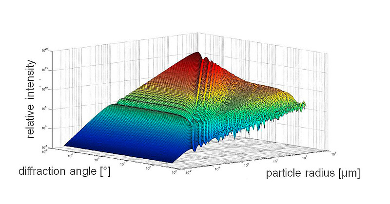
Figure 8: Expected intensities of light at different diffraction angles for particles of various sizes.
Diffraction data analysis theory
Two different theories are used for the analysis of laser diffraction raw data, namely Fraunhofer and Mie (Figure 9). Both assume a spherical particle shape. Fraunhofer theory is simpler, as it does not take into account phenomena like absorption, refraction, reflection, or scattering of light. It works well for large and/or opaque particles, and doesn’t require any knowledge of the particle’s optical properties. Mie theory, however, does consider other light scattering phenomena, and consequently requires knowledge of the particle’s refractive index and absorption coefficient for the particular wavelength. As a general principle, it is always preferable to use Fraunhofer theory as a default, rather than using Mie theory with possibly inaccurate values for the particle’s optical properties.
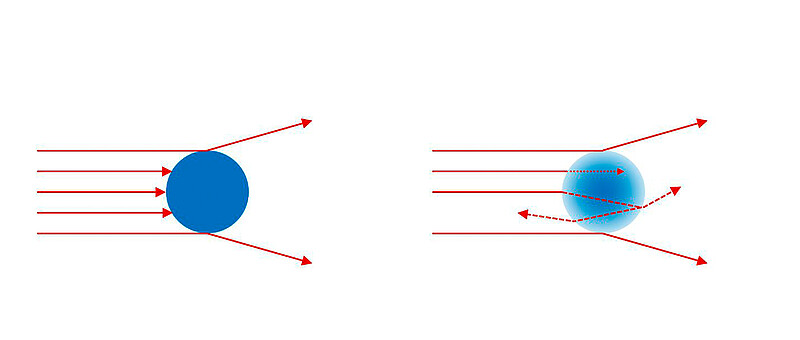
Figure 9: Illustration of the difference between Fraunhofer (left) and Mie diffraction theory (right). Large and opaque particles are usually analyzed using Fraunhofer diffraction theory. Mie theory also considers other optical phenomena in addition to diffraction.
Particle size distribution
Laser diffraction gives an estimation of the percentage of particles belonging to a certain size class. Size classes are groups of particles of similar sizes and each size class is assigned two different diameters (Figure 10).
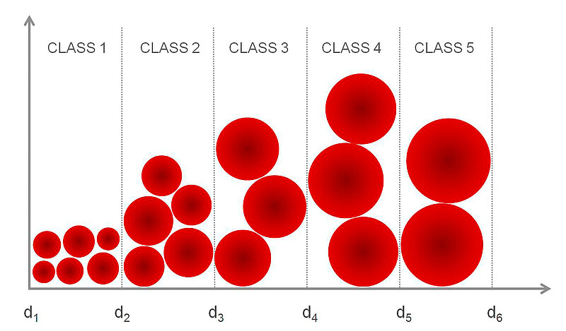
Figure 10: Illustration of size classes and how they are defined by two diameters.
A typical result of a laser diffraction measurement is shown in Figure 11. The basic particle size distribution might have one or more peaks for size classes, which indicate the most common particle sizes. The Dmode value defines the position of the highest peak. However, there might be more peaks or the peak might be weakly defined (e.g. spikey, flat, etc.), so peak values are rather unreliable. For this reason, usually the cumulative distribution is analyzed. To get this distribution, values for all previous classes are added to the next. This is done either from the smallest to the biggest diameter (called the "undersize curve") or in the opposite direction (called the "oversize curve"). In either direction, the cumulative curve always ranges from 0 % to 100 %, with the middle point D50 being the most commonly reported result of particle sizing by laser diffraction. D50 defines the point where 50 % of the particles are smaller and 50 % bigger than that certain diameter. The beginning and end of the distribution are commonly defined by D10 and D90, although other D values can be used to define the cumulative distribution as well (e.g. D1 or D99).
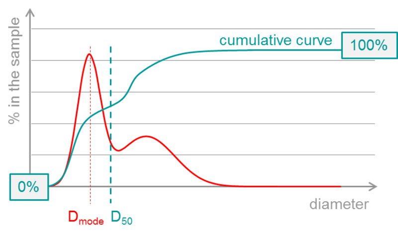
Figure 11: Typical result of a laser diffraction particle size measurement. The red curve is the basic particle size distribution, with the Dmode value defining the position of the peak. The cumulative curve ("undersize", here shown in turquoise) has its middle point at D50 – it being the single most common result of particle sizing by laser diffraction.
In laser diffraction the percentages of the particle sizes in the sample are typically given in volume (volume-based distribution). Alternatively, the relative proportions of particle sizes can also stand for the surface of the particles or number-based distributions. Since the theories used for laser diffraction assume spherical particles, the representations in surface and number are made by applying a geometrical calculation (for the surface area and volume of a sphere) to the volume-based result.
Conclusion
Particle size is a common quality control parameter, affecting both the production process and the final properties of a product. Laser diffraction is a valuable tool for particle sizing, from the sub-micron to the millimeter range. The increasing popularity of this method is due to its high repeatability combined with its fast and easy measurement technique that requires low sample amounts. Laser diffraction is a relative method which uses the optical behavior of particles to derive their sizes. In order to do so, the analysis theory assumes that the measured particles are spherical and reports their diameter. Obviously, for non-spherical particles this leads to a deviation from their real sizes. However, as the shape-caused error remains consistent, this makes laser diffraction a highly reliable quality control tool.
Further references
- Xu, R. (2002). Particle Characterization: Light Scattering Methods. Dordrecht: Springer Netherlands, 111-181
- Merkus, H. (2009). Particle Size Measurements. Dordrecht: Springer Netherlands, 259-285
- Bohren, C. and Huffman, D. (2007). Absorption and Scattering of Light by Small Particles.Weinheim: Wiley-VCH Verlag GmbH & Co. KGaA, 381-428
- ISO 13320:2009, Particle size analysis - Laser diffraction methods