Particle size distribution
Particle size is one of the most important characteristics of particulate materials. It directly affects many material properties, from the accessibility of minerals during processing, to the absorption kinetics of drugs, and the mouthfeel of foods. In industry, the aim of particle size measurement is first and foremost to find a correlation between the particle size distribution and the property of interest (e.g., mouthfeel, reactivity, bioavailability, sintering behavior, etc.). This information can then be used to modify the manufacturing processes that impact particle size and, ultimately, to use particle size distribution as a quality control parameter.
Thanks to modern instrumentation, measuring the particle size distribution of a substance is an easy and straightforward task, which can often be performed in less than a minute. A large variety of techniques are available, which deliver an equally large variety of results in the form of means, averages, modes, and other parameters. The key to understanding the results is to first know the meaning of these parameters.
In this article, we introduce the basic terms and their use in particle size analysis and discuss the advantages and disadvantages of using single parameters vs. multiple parameters to characterize particle size distribution.
Describing the particle size distribution with a single parameter
Obtaining a meaningful description of a particulate system with many different particle sizes and shapes using just one or two parameters is challenging. To deliver useful information, the chosen parameter should be easy to calculate, be specific enough, and have a direct connection to the substance’s property of interest.
Different measurement techniques “see” the particles in a different way, which translates to a different weighting as the result. The main weighting models used to analyze particle size distribution are:
- Number-weighted distribution (% number)
- Surface-weighted distribution (% in surface)
- Volume-weighted distribution (% in volume)
As an example, a microscope sees the diameter of each individual particle, so this technique will deliver a number-weighted result. In contrast, the diffraction of light is proportional to the volume of the particle, therefore techniques such as laser diffraction or X-ray diffraction deliver volume-weighted results.
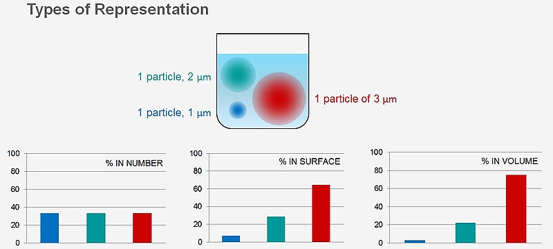
Figure 1 shows an example of how the particle size distribution (PSD) of a mixture containing 1 µm, 2 µm, and 3 µm particles would look like in different weightings. The main difference between these weightings is the representation of the fine fraction compared to the coarse fraction. Number weighting gives equal representation to the fine and the coarse fraction. In contrast, in the volume-weighted results a few large particles might outweigh numerous smaller particles.
Both representations have their merits depending on what is required from a measurement. For someone working in the mining industry, it is important to know the size of the particles in a given volume, while in microbiology, where individual cells are counted, the number-based distribution is preferred. An operator working on catalysts will certainly choose the surface-weighted distribution as the catalyst’s activity depends on the extend of its contact surface with the reactant.
Different particle sizing techniques will also give results that are intrinsically of a specific weighting, as shown in Table 1 below.
| Weighting | Measurement technique |
|---|---|
| Number-weighted distribution (% number) | Microscopy, dynamic image analysis |
| Surface-weighted distribution (% in surface) (% in surface) | Gas absorption |
| Volume-weighted distribution (% in volume) | Sedimentation, laser diffraction, X-ray diffraction |
| Intensity-weighted distribution (% in intensity) | Dynamic light scattering (DLS) |
The intensity-weighted distribution is specific to the dynamic light scattering (DLS) technique. In that case, the results are expressed as a measure of the intensity fluctuations of the light scattered by the particle. This is considered to give even greater weighting to the large particles than the volume-weighted distribution, so that native DLS particle size distributions are even more skewed towards large particles than laser diffraction results.
The remaining sections of this article look at the selection of options to visualize, analyze, and compare particle size distributions by example of a measurement performed via the laser diffraction technique.
Using laser diffraction to obtain a single parameter for quality control
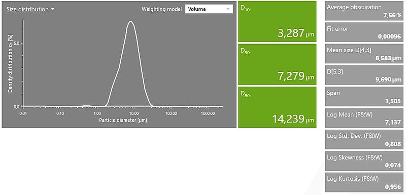
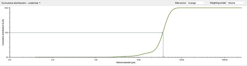
When using laser diffraction, the two most common visual representations are the density or frequency distribution (q3), see Figure 2, and the cumulative curve (Q3), shown in Figure 3. The former displays the probability of finding a particle with diameter d in the population, while the latter shows the percentage of particles which are smaller (undersize) or bigger (oversize) than diameter d. The two are in strong mathematical correlation, as the cumulative curve is a simple integral of the frequency curve:
$$Q_3(r)=\int_{0}^{r} q_3(r) dr$$
Graphical depiction is practical, as it gives lots of information at a glance. A few examples are the modality, the relative ratios of the particle populations, the broadness, and the general shape of the distribution. Although a visual input is fast and convenient, for documentation and comparison purposes numerical values are indispensable. The three most important options for describing a particle size distribution by a single parameter are:
- the mode
- the median
- the mean
The mode
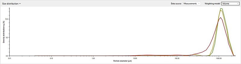
The mode is defined as the most commonly occurring size. It is the peak position on the frequency distribution curve. This frequency distribution curve is a straightforward figure for strictly monomodal (having only one peak) and narrow samples, such as latex beads, or monodisperse (containing only particles of very similar sizes) nanoparticle populations. However, its limitations become clear once more than one particle population is present in the sample (bimodal or polymodal substances) or when characterizing polydisperse samples. Figure 3 shows an example with three samples, all of which have a very similar mode although the particle size distribution of the three samples is clearly different.
The median
The median is the value separating the higher half of the data from the lower half. It is the determined particle size from which half of the particles are smaller and half are larger. This is also called D50 (see Figure 1). The median is easy to determine from the cumulative distribution curve (s. Figure 4). However, it has the same problem as the mode: Several distributions may have the same median; therefore it is not reliable as a single figure.
The mean
According to ISO 9276-2, [1] the general definition of mean particle size according to the Moment-Ratio-notation is:
$$\bar{D}_{[p,q]}=(\frac{\sum n_iD_i^p}{\sum n_iD_i^q})^{1/(p-q)} $$, if $$p\neq\ q$$
…where ni is the frequency of occurrence of particles in size class i, having a mean Di diameter.
The following diameters are commonly used in laser diffraction (Table 2):
| Mean diameter name | Moment-Ratio notation | Formula | Main applications |
| Number-weighted mean | D[1,0] | $$D_{[1,0]}=\frac{\sum n_iD_i}{\sum n_i} $$ | Biological applications: viruses, blood cell counting Comparison of laser diffraction results to results obtained by optical methods (e.g., microscopy). |
| Surface-weighted (or Sauter) mean | D[3,2] | $$D_{[3,2]}=\frac{\sum n_iD_i^3}{\sum n_iD_i^2} $$ | Fluid dynamics, catalysis, fuel combustion |
| Volume-weighted (or De Brouckere) mean | D[4,3] | $$D_{[4,3]}=\frac{\sum n_iD_i^4}{\sum n_iD_i^3} $$ | Mining, comminution, mineral processing, building materials |
| Volume-weighted mean area size | D[5,3] | $$D_{[5,3]}=(\frac{\sum n_iD_i^5}{\sum n_iD_i^3})^{1/2} $$ | Emulsion science, in particular to describe the homogenization efficiency of milk. (D5,3 )2 is also termed “creaming parameter,” or H, according to Walstra [2]. |
Other methods
Additionally, several methods were developed in the 20th century in order to provide a single measure for the quality check of products in the mining, milling, and grinding industries. The two most prominent examples are the Rosin-Rammler (RR) model and the Gates-Gaudin-Schuchmann (GGS) model. Both of these provide a linearization of the distribution through a logarithmic calculation and provide a more sensitive median (D63.5).
Describing the particle size distribution by multiple parameters
A single number is a valuable piece of information for quality control purposes, e.g. when checking for differences in production batches. However, it does not deliver information about the source of the deviation, such as the shape, broadness, modality, etc. A deeper investigation into, and understanding of, the source of differences call for a multiparameter description of the particle size distribution. The following parameters are used in particle sizing techniques.
D-values
The most common values used in several particle sizing techniques are the D-values. These are related to the cumulative distribution and are only meaningful followed by a number, e.g. Dx. Both undersize and oversize D-values can be defined (just like the cumulative curve can be undersize or oversize). If not stated otherwise, the standard is the undersize D-value which means that in general Dx gives the diameter of which x percentage of the particles are smaller. The three most often used D-values are D10, D50, and D90 (see Figure 2), but custom D-values can be found for particular applications (e.g. IV Insulin).
Even though D-values are the most often used results due to their convenience and easy to understand definition, they are typically meant for quality control purposes as an alternative to the single parameter but more calculation-heavy RR (Rosin-Rammler) or GGS (Gates-Gaudin-Schuchmann) method.
Span
In most cases a useful description of a particle size distribution also calls for a way to describe the shape of the distribution. An important measure of any statistical distribution is the width or broadness. In laser diffraction an often-used measure is the span. It is calculated in general by the following formula:
$$ Span = \frac{D_{90} - D_{10}}{D_{50}} $$
However, some custom-defined spans exist for specific applications.
Folk & Ward parameters
Some samples, such as soil and geological samples, have a large variety of grain sizes and are classified accordingly. Their particle size distribution is often complex with very broad, multimodal distribution. For the analysis of such samples Folk and Ward (F&W) proposed a statistical grain-size analysis method [Ref: (R.L. Folk, 1957), AR: Soil].
At the core of the method is the conversion of the particle size distribution from millimeters to the phi scale by the following formula:
$$ \phi = -\log_{2}d $$
Followed by the calculation of a set of parameters:
- Median: see above. Measured in phi units
- Mean: definition as above, however Folk proposed his own formula (R.L. Folk, 1957):
$$ M_z = \frac{\phi_{16} + \phi_{50} + \phi_{84}}{3} $$ The mean is also measured in phi units and is the most widely used of all the parameters. - Skewness: Measure of the asymmetry of the distribution around its peak. It is determined by the equation:
$$ sk_1 = \frac{\phi_{16} + \phi_{84} - 2\phi_{50}}{2(\phi_{84} - \phi_{16})} + \frac{\phi_{5} + \phi_{95}-2\phi_{50}}{2(\phi_{95}-\phi_{5})} $$ The skewness is also given in phi units. There are other means of calculating the skewness. However, the formula proposed by Folk also takes the “tails” into consideration. Perfectly symmetrical distributions have a skewness of 0.00. A positive skew represents an increased fine portion (“tail” on the left), while a negative skew indicates a shift to the coarse materials (“tail” on the right). Folk also suggested a classification:- ±0.1 is nearly symmetrical
- -0.10 to -0.30 is coarse-skewed and +0.1 to +0.3 is fine-skewed
- -0.30 to -1.00 is strongly coarse skewed and +0.3 to +1.0 is strongly fine-skewed.
-
Kurtosis: Measure of the deviation from the normal (Gaussian) distribution or in other words the “peakedness”. The formula proposed by Folk is:
$$ k_g=\frac{\phi_{95} - \phi_{5}}{2.44(\phi_{75}-\phi_{25})} $$ Kurtosis is measured in phi units as well. It can be used to determine the number of outliers in the sample. A perfectly Gaussian curve has a kurtosis of 1.00 and is also called mesokurtic. If the sample is more sharp-peaked, hence less outliers are present, then the kurtosis is higher than 1.00 and it is called leptokurtic. If the sample curve is more flat-peaked, meaning there are a large number of outliers in the sample, the value is smaller than 1.00. Such a distribution is called platykurtic.
Phi units furthermore have the advantage of providing an easy-to-read scale of size classes for the classification of soil types starting from boulders (ϕ > -8) down to clay (ϕ < 8).
Conclusion
Analyzing the particle size distribution is a convenient tool for quality control as well as research and development. Through the careful and mindful selection of the right measurement method, weighting model, mode, and further parameters, you can extract crucial information about a material’s given property.
Read more about the importance of particle size analysis for specific sample groups:
Read more about the different particle analysis techniques:
References
[1] I. 9276-2:2014. 2014. "Representation of Results of Particle Size Analysis — Part 2: Calculation of Average Particle Sizes/Diameters and Moments from Particle Size Distributions."
[2] Walstra, P., and H. Oortwijn. 1975. "Effect of Globule Size and Concentration on Creaming in Pasteurized Milk." Netherlands Milk and Dairy Journal, vol. 29: 263–278.
[3] Folk, R. L., and W. C. Ward. 1957. "Brazos River Bar: A Study in the Significance of Grain Size Parameters." Journal of Sedimentary Petrology, vol. 27: 3–26.
[4] Typical results of a particle size analysis by laser diffraction (CC BY license)