Dynamic light scattering: Principles and basics
The method of dynamic light scattering (DLS) is the most common measurement technique for particle size analysis in the nanometer range. In this article we describe the theory as well as the basic DLS setup and explain how the particle size is determined. Further, the typical outcome of a DLS analysis is shown and practical tips on measurement settings and data verification are included.
Theoretical background of dynamic light scattering
Dynamic light scattering (DLS) is based on the Brownian motion of dispersed particles. When particles are dispersed in a liquid they move randomly in all directions. The principle of Brownian motion is that particles are constantly colliding with solvent molecules. These collisions cause a certain amount of energy to be transferred, which induces particle movement. The energy transfer is more or less constant and therefore has a greater effect on smaller particles. As a result, smaller particles are moving at higher speeds than larger particles. If you know all other parameters which have an influence on particle movement, you can determine the hydrodynamic diameter by measuring the speed of the particles.
The relation between the speed of the particles and the particle size is given by the Stokes-Einstein equation (Equation 1). The speed of the particles is given by the translational diffusion coefficient D. Further, the equation includes the viscosity of the dispersant and the temperature because both parameters directly influence particle movement. A basic requirement for the Stokes-Einstein equation is that the movement of the particles needs to be solely based on Brownian motion. If there is sedimentation, there is no random movement, which would lead to inaccurate results. Therefore, the onset of sedimentation indicates the upper size limit for DLS measurements. In contrast, the lower size limit is defined by the signal-to-noise ratio. Small particles do not scatter much light, which leads to an insufficient measurement signal.
$D= \frac{k_BT}{6\pi\eta R_H}$
Equation 1: The Stokes-Einstein equation
D Translational diffusion coefficient [m²/s] – “speed of the particles”
kB Boltzmann constant [m²kg/Ks²]
T Temperature [K]
h Viscosity [Pa.s]
RH Hydrodynamic radius [m]
The basic DLS setup
The basic setup of a DLS instrument is shown in Figure 1. A single frequency laser is directed to the sample contained in a cuvette. If there are particles in the sample, the incident laser light gets scattered in all directions. The scattered light is detected at a certain angle over time and this signal is used to determine the diffusion coefficient and the particle size by the Stokes-Einstein equation.
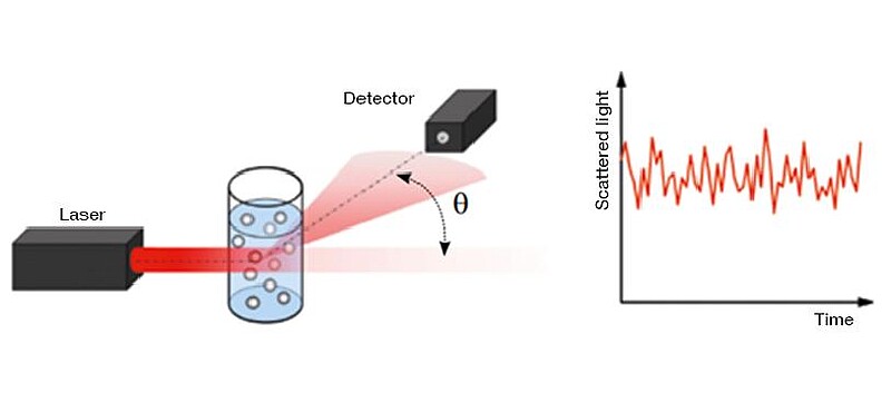
Figure 1: Basic setup of a DLS measurement system. The sample is contained in a cuvette. The scattered light of the incident laser can be detected at different angles.
The incident laser light is usually attenuated by a gray filter which is placed between the laser and the cuvette. The filter settings are either automatically adjusted by the instrument or can be set manually by the user. When turbid samples are measured the detector would not be able to process the amount of photons. Therefore, the laser light is attenuated to receive a sufficient but processable signal at the detector.
Modern DLS instruments include two, or in the case of Litesizer™ 500 three, detection angles for particle size measurements. Depending on the turbidity of the sample, side scattering (90°) or back scattering (175°) is more suitable. A forward angle (15°) can be used to monitor aggregation. For more information on this subject, see section "Choosing the rightmeasurement angle".
Intensity trace and correlation function
The scattered light is detected over a certain time period in order to monitor the movement of the particles. The intensity of the scattered light is not constant but will fluctuate over time. Smaller particles, which are moving at higher speeds, show faster fluctuations than larger particles. On the other hand, larger particles result in higher amplitudes between the maximum and minimum scattering intensities, as shown in Figure 2 (upper panels). This initial intensity trace is further used to generate a correlation function (Fig. 2, lower panels). In general, the correlation function describes how long a particle is located at the same spot within the sample. At the beginning the correlation function is linear and almost constant, indicating that the particle is still at the same position as it was the moment before. Later, you can see an exponential decay of the correlation function, which means that the particle is moving. If there is no similarity to the initial spot, the correlation function shows a linear behavior again. This part of the correlation function is known as the baseline. The information of the size-dependent movement is included in the decay of the correlation function. The decay represents an indirect measure of the time that the particles need to change their relative positions. Small particles move quickly so the decay is fast. Larger particles move more slowly and therefore the decay of the correlation function is delayed.

Figure 2: Differences in the intensity trace and correlation function of large and small particles. Smaller particles show faster fluctuations of the scattered light and a faster decay of the correlation function.
In fact, the correlation function is a mathematical description of the fluctuations of the scattered light. It is used to determine the translational diffusion coefficient. To do this, the intensity of the scattered light at a time t is compared with the intensity of the same intensity trace shifted by the delay time ꞇ (tau). This abstract mathematical concept is visualized in Figure 3. It shows the same intensity trace as recorded during the measurement and shifted for different delay times ꞇ. Different delay times are marked by a different color. Each single value of G2 is then obtained by adding together the product of two values at the same time of these two intensity traces, which is indicated by the colored connection for one position per delay time. Doing this for different delay times results in the desired correlation function. These calculations are done in real time and plotted over a logarithmic time axis. Cumulant algorithms are used in order to fit the correlation function, which is an ISO-standardized procedure. The diffusion coefficient is determined from the cumulant algorithm; the hydrodynamic diameter (i.e. particle size) is further obtained by the already discussed Stokes-Einstein equation.
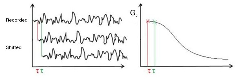
Figure 3: Translating the intensity trace (left panel) into a correlation function (right panel)
Measurement results
As described above, the particle size of the sample is not measured directly but is based on the movement of the particles. The term hydrodynamic diameter refers to the particle size of smooth, spherical particles which diffuse at the same speed as the particles of the sample. This has to be kept in mind when the results of DLS measurements are compared with other techniques, which refer to different physical parameters of the sample.
The polydispersity index (PDI) is given in order to describe the broadness of the particle size distribution. The polydispersity index is also calculated by the cumulant method. A value below 10 % reflects a monodisperse sample and indicates that all of the measured particles have almost the same size. However, the polydispersity index does not provide any information about the shape of the size distribution or the ratio between two particle fractions. This information is given by the particle size distribution chart, which is part of the one-page workflow of the Litesizer™ 100/500 software (see Figure 4).
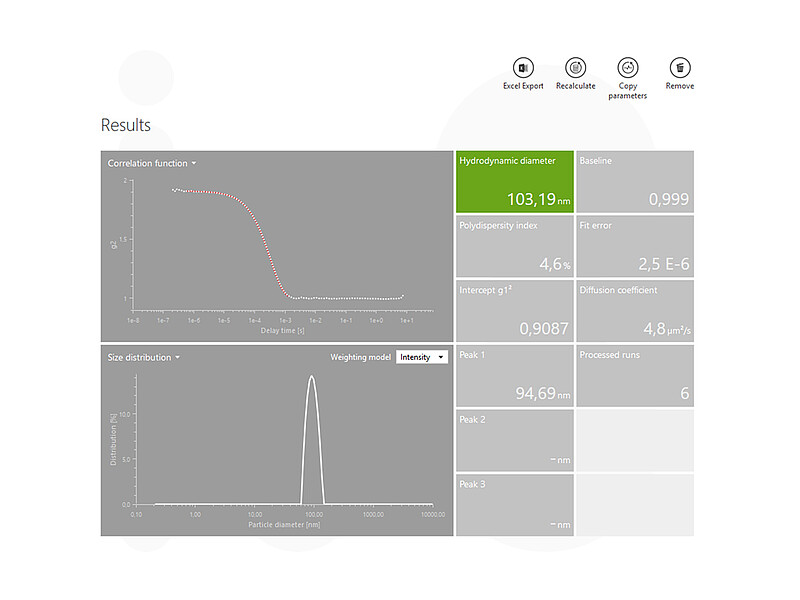
Figure 4: Typical result overview of a DLS measurement. The initial results (hydrodynamic diameter, polydispersity index) are displayed as well as information about the correlation function (baseline, intercept, etc.). The particle size distribution chart gives further information about different size populations within the measured sample.
As the results of DLS measurements are intensity-based (the intensity fluctuations over time are detected) this is the primary weighting model displayed in a DLS software. The intensity-based distribution can be re-calculated to a volume- and number-based distribution. For this, the material refractive index and the absorbance of the measured sample at the wavelength of the laser need to be known. Intensity-based techniques show an emphasis on larger particles (they scatter more light than smaller particles). Volume- and number-based distributions will show a tendency to smaller particle fractions. It is important to note that all three size distributions are just different representations of the same physical reality of a distribution of differently sized particles. The initial results from a DLS measurement (hydrodynamic diameter and the polydispersity index) are related to the intensity-weighted particle size distribution defined by ISO 224121. Therefore, these values will not change, if different weighting models are selected.
Verifying the data quality of DLS measurements
During a measurement, DLS software shows live signals of the intensity trace as well as of the generated correlation function. These signals provide a lot of information on the data quality. The intensity trace will show regular fluctuations of the scattered light, if monodisperse samples are measured. If sharp spikes are observed, it is most likely that the sample is contaminated by dust particles or aggregates. Another effect which can be observed is that the intensity trace ramps up or down. A steady increase or decrease in the intensity trace might show a thermal gradient during the measurement time. Further, a steady increase can indicate aggregation and a steady decrease may be due to sedimentation.
The correlation function gives information about the signal-to-noise ratio as well as on the presence of dust particles or aggregates. For a monomodal dispersion the correlation function should be smooth and with a single exponential decay. A non-linear baseline including several bumps indicates the presence of dust particles or aggregates. The signal-to-noise ratio can be evaluated from the plateau value of the correlation function at small delay times, the so-called intercept. If there is not enough signal collected, the difference will be low and no meaningful correlation function can be generated. This might be the case, if very small particles are measured or the particle concentration is too low.
Choosing the right measurement angle
Modern DLS instruments provide different detection angles for particle size measurements (typically at 15°, 90°, and 175°). Litesizer™ 500 uses the included transmittance measurement for automatic angle selection. Side- or back scattering is automatically selected by the instrument depending on which is the most suitable angle for the measured sample.
If the measurement is performed at 175°, this is back scattering. At this angle the scattering volume (the volume where the incident laser beam and the detected light overlap) is near the front cuvette wall. That means the path length of the laser within the sample is very short. This serves as an ideal setup for highly concentrated and turbid samples as it minimizes the effect of multiple scattering. Multiple scattering means that the light is scattered at more than one particle, which can interfere with the measurement signal. In order to further minimize the path length of the laser the focus position can also be adjusted (Figure 5).

Figure 5: DLS instruments can adjust the focus position by moving a focusing lens. If the focus position is near the front cuvette wall, multiple scattering events can be minimized. The overlap of the incident laser beam and the scattered light is called scattering volume.
Side scattering at 90° is the angle of choice for weakly scattering samples of small particles because the flare created by the laser at the cuvette wall is blocked from entering the detection optics and this leads to a cleaner result. Therefore, measurements done using the side angle are less sensitive to dirt and scratches on the cuvette wall.
The forward angle at 15° is used to monitor aggregation or if a sample of smaller particles contains a few large particles. As larger particles scatter more light in the forward direction than in other directions these particles are emphasized at this angle. By comparing the results with other measurement angles the presence of aggregates can be monitored.
Summary and conclusion
Dynamic light scattering is a well-established, standardized technique for particle size analysis in the nanometer range and has been used for about 40 years. DLS provides information on the mean particle size as well as on particle size distribution. It covers a broad size range from the lower nanometer range up to several micrometers. Only low sample volumes are required and the sample can be re-used after the measurement. Instruments normally also provide Electrophoretic Light Scattering (ELS) and Static Light Scattering (SLS) for zeta potential analysis and determination of the molecular mass in order to serve as an ideal tool for extensive particle analysis.
Read more about detection angles used by DLS instruments here.
For more information about Litesizer DLS instruments, see here.
References
1. ISO 22412:2017. Particle Size Analysis – Dynamic Light Scattering (DLS). International Organization for Standardization.